Download

1 / 21
210 likes | 239 Views
Learn about parallel algorithms in the PRAM model, synchronization, list ranking, prefix computation, and finding roots. Discover the EREW and CRCW models, synchronization challenges, and efficient algorithms.

E N D
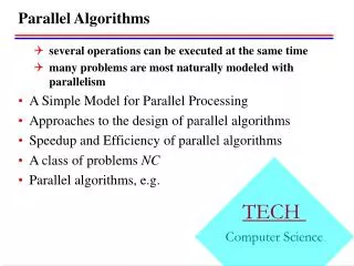
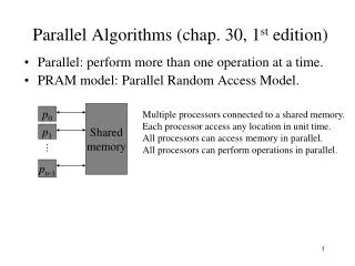
Parallel Algorithms (chap. 30, 1st edition) • Parallel: perform more than one operation at a time. • PRAM model: Parallel Random Access Model. Shared memory p0 Multiple processors connected to a shared memory. Each processor access any location in unit time. All processors can access memory in parallel. All processors can perform operations in parallel. p1 pn-1
Concurrent vs. Exclusive Access • Four models • EREW: exclusive read and exclusive write • CREW: concurrent read and exclusive write • ERCW: exclusive read and concurrent write • CRCW: concurrent read and concurrent write • Handling write conflicts • Common-write model: only if they write the same value. • Arbitrary-write model: an arbitrary one succeeds. • Priority-write model: the one with smallest index succeeds. • EREW and CRCW are most popular.
Synchronization and Control • Synchronization: • A most important and complicated issue • Suppose all processors are inherently tightly synchronized: • All processors execute the same statements at the same time • No race among processors, i.e, same pace. • Termination control of a parallel loop: • Depend on the state of all processors • Can be tested in O(1) time.
Pointer Jumping –list ranking • Given a single linked list L with n objects, compute, for each object in L, its distance from the end of the list. • Formally: suppose next is the pointer field • d[i]= 0 if next[i]=nil • d[next[i]]+1 if next[i]nil • Serial algorithm: (n).
List ranking –EREW algorithm • LIST-RANK(L) (in O(lg n) time) • for each processor i, in parallel • doifnext[i]=nil • thend[i]0 • elsed[i]1 • while there exists an object i such that next[i]nil • dofor each processor i, in parallel • do ifnext[i]nil • then d[i] d[i]+ d[next[i]] • next[i] next[next[i]]
3 4 6 1 0 5 (a) 1 1 1 1 1 0 4 4 3 2 1 0 5 4 3 2 1 0 List-ranking –EREW algorithm 3 4 6 1 0 5 (b) 2 2 2 2 1 0 3 4 6 1 0 5 (c) 3 4 6 1 0 5 (d)
List ranking –correctness of EREW algorithm • Loop invariant: for each i, the sum of d values in the sublist headed by i is the correct distance from i to the end of the original list L. • Parallel memory must be synchronized: the reads on the right must occur before the wirtes on the left. Moreover, read d[i] and then read d[next[i]]. • An EREW algorithm: every read and write is exclusive. For an object i, its processor reads d[i], and then its precedent processor reads its d[i]. Writes are all in distinct locations.
LIST ranking EREW algorithm running time • O(lg n): • The initialization for loop runs in O(1). • Each iteration of while loop runs in O(1). • There are exactly lg n iterations: • Each iteration transforms each list into two interleaved lists: one consisting of objects in even positions, and the other odd positions. Thus, each iteration double the number of lists but halves their lengths. • The termination test in line 5 runs in O(1). • Define work =#processors running time. O(n lg n).
Parallel prefix on a list • A prefix computation is defined as: • Input: <x1, x2, …, xn> • Binary associative operation • Output:<y1, y2, …, yn> • Such that: • y1= x1 • yk= yk-1 xk fork=2,3, …,n, i.e, yk= x1 x2 … xk . • Suppose <x1, x2, …, xn> are stored orderly in a list. • Define notation: [i,j]= xi xi+1 … xj
Prefix computation • LIST-PREFIX(L) • for each processor i, in parallel • doy[i] x[i] • while there exists an object i such that next[i]nil • dofor each processor i, in parallel • do ifnext[i]nil • then y[next[i]] y[i] y[next[i]] • next[i] next[next[i]]
x5 x1 x2 x4 x6 x3 (a) [1,1] [2,2] [4,4] [5,5] [3,3] [6,6] x1 x1 x1 x6 x6 x6 x2 x2 x2 x5 x5 x5 x3 x3 x3 [1,1] [1,2] [1,3] [1,4] [1,5] [1,6] Prefix computation –EREW algorithm x4 (b) [1,1] [1,2] [2,3] [3,4] [4,5] [5,6] (c) [1,1] [1,2] [1,3] [1,4] [2,5] [3,6] (d)
Find root –CREW algorithm • Suppose a forest of binary trees, each node i has a pointer parent[i]. • Find the identity of the tree of each node. • Assume that each node is associated a processor. • Assume that each node i has a field root[i].
Find-roots –CREW algorithm • FIND-ROOTS(F) • for each processor i, in parallel • doifparent[i] = nil • thenroot[i]i • while there exist a node i such that parent[i] nil • dofor each processor i, in parallel • do if parent[i] nil • then root[i] root[parent[i]] • parent[i] parent[parent[i]]
Find root –CREW algorithm • Running time: O(lg d), where d is the height of maximum-depth tree in the forest. • All the writes are exclusive • But the read in line 7 is concurrent, since several nodes may have same node as parent. • See figure 30.5.
Find roots –CREW vs. EREW (lg n) • How fast can n nodes in a forest determine their roots using only exclusive read? Argument: when exclusive read, a given peace of information can only be copied to one other memory location in each step, thus the number of locations containing a given piece of information at most doubles at each step. Looking at a forest with one tree of n nodes, the root identity is stored in one place initially. After the first step, it is stored in at most two places; after the second step, it is Stored in at most four places, …, so need lg n steps for it to be stored at n places. So CREW: O(lg d) and EREW: (lg n). If d=2(lg n), CREW outperforms any EREW algorithm. If d=(lg n), then CREW runs in O(lg lg n), and EREW is much slower.
A[j] 5 6 9 2 9 m 5 F T T F T F 6 F F T F T F 9 F F F F F T 2 T T T F T F 9 F F F F F T A[i] max=9 Find maximum – CRCW algorithm • Given n elements A[0,n-1], find the maximum. • Suppose n2 processors, each processor (i,j) compare A[i] and A[j], for 0 i, j n-1. • FAST-MAX(A) • nlength[A] • fori 0 ton-1, in parallel • dom[i] true • fori 0 ton-1 and j 0 ton-1, in parallel • do ifA[i] < A[j] • thenm[i] false • fori 0 ton-1, in parallel • doifm[i] =true • thenmax A[i] • returnmax The running time is O(1). Note: there may be multiple maximum values, so their processors Will write to max concurrently. Its work = n2 O(1) =O(n2).
Find maximum –CRCW vs. EREW • If find maximum using EREW, then (lg n). • Argument: consider how many elements “think” that they might be the maximum. • First, n, • After first step, n/2, • After second step n/4. …, each step, halve. • Moreover, CREW takes (lg n).
Stimulating CRCW with EREW • Theorem: • A p-processor CRCW algorithm can be no more than O(lg p) times faster than a best p-processor EREW algorithm for the same problem. • Proof: each step of CRCW can be simulated by O(lg p) computations of EREW. • Suppose concurrent write: • CRCW pi write data xi to location li, (li may be same for multiple pi ‘s). • Corresponding EREW pi write (li, xi) to a location A[i], (different A[i]’s) so exclusive write. • Sort all (li, xi)’s by li’s, same locations are brought together. in O(lg p). • Each EREW pi compares A[i]= (lj, xj), and A[i-1]= (lk, xk). If ljlkor i=0, then EREW pi writes xj to lj. (exclusive write). • See figure 30.7.
CRCW vs. EREW • CRCW: • Some says: easier to program and more faster. • Others say: The hardware to CRCW is slower than EREW. And One can not find maximum in O(1). • Still others say: either EREW or CRCW is wrong. Processors must be connected by a network, and only be able to communicate with other via the network, so network should be part of the model.