Lecture 4: Boundary Value Problems
Lecture 4: Boundary Value Problems. Instructor: Dr. Gleb V. Tcheslavski Contact: gleb@ee.lamar.edu Office Hours: Room 2030 Class web site: www.ee.lamar.edu/gleb/em/Index.htm. What will we learn.

Lecture 4: Boundary Value Problems
E N D
Presentation Transcript
Lecture 4: Boundary Value Problems Instructor: Dr. Gleb V. Tcheslavski Contact:gleb@ee.lamar.edu Office Hours:Room 2030 Class web site:www.ee.lamar.edu/gleb/em/Index.htm
What will we learn So far, we considered fields in an infinite space. In practice, however, we often encounter situations when fields live in a finite space consisting of bounded regions with different electromagnetic properties. We have learned that an electrostatic field could be created from a charge distribution. The electric potential can be obtained in terms of charge distributions via Poisson’s equation. Now, we will examine how to solve such equations in general.
Boundary conditions We restrict our discussion to a 2D case and Cartesian coordinates With respect to the interface between two boundaries, an EM field can be separated into a parallel (tangential) and a perpendicular (normal) components
Boundary conditions: normal components Normal components for the displacement flux density D and the magnetic flux density B “Pillbox” Thickness: Cross-section area s
Boundary conditions: normal components (cont) We assume that there is a charge distributed along both sides of the interface and has a total charge density of s. Electric field from the Gauss’s law: (4.5.1) (4.5.2) Magnetic field: (4.5.3) (4.5.4)
Boundary conditions: tangential components Electric field: the total work is (4.6.1) Assume that z portions can be neglected; two other edges: (4.6.2)
Boundary conditions: tangential components (cont) For the magnetic field, Ampere’s law: (4.7.1) surface current density Here, we again neglected integration over the top and bottom edges. (4.6.5)
Boundary conditions: Example The surface current with a density Js = 20uyA/m is flowing along the interface between two homogeneous, linear, isotropic materials with r1 = 2 and r2 = 5. H1 = 15ux + 10uy + 25uzA/m. Find H2. 1. Normal component: 2. Tangential component: 3. There is no change in the y-component of the magnetic field. WHY?
Boundary with ideal conductor Since the tangential electric field must be continuous, and accounting for the Ohm’s law, it must be a tangential current approaching infinity! Therefore, the tangential current density and tangential component of E must be zero at the interface with a perfect conductor. Ideal conductors are equipotential. The consequence: if we place a point charge above an ideal conductor, it will create an electric field that would be entirely in a radial direction. Therefore, the tangential component of E will be zero just beneath the charge. In order to satisfy the “zero tangential component requirement” at the other points of the surface, we assume that so called “image charge” exists inside the conductor.
Poisson’s and Laplace’s equations The Gauss’s law in differential form: (4.10.1) Electrostatic field is conservative: (4.10.2) Therefore, E is a gradient of electric potential: (4.10.3) Combining (4.10.1) and (4.10.3), the Poisson’s equation: (4.10.4) If the charge density in the region is zero, the Laplace’s equation: (4.10.5)
Poisson’s and Laplace’s equations From non-existence of magnetic monopole: (4.11.1) A vector magnetic potential such that: (4.11.2) The Ampere’s law in differential form: (4.11.3) Therefore: (4.11.4) Via the vector identity, the Coulomb’s gauge is: (4.11.5) Similarly to the Poisson’s equation: (4.11.6) In the CCS: (4.11.7)
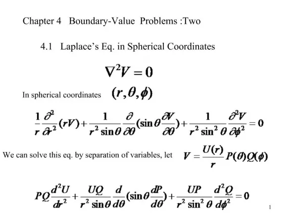
Poisson’s and Laplace’s equations Recall that the Laplacian operator in different CSs: 1. Cartesian: (4.12.1) 2. Polar: (4.12.2) 3. Spherical: (4.12.3)
Poisson’s equation: Example Show that the 2D potential distribution Satisfies the Poisson’s equation Let us evaluate the Laplacian operator in the Cartesian CS: Therefore: At this point, we derived the Poisson’s and Laplace’s equations in 3D. Next, we will attempt to solve them to find a potential.
x = 0 x = x0 Analytical solution in 1D – Direct integration Calculate the potential variation between two infinite parallel metal plates in a vacuum. We assume no resistance, therefore, no variation in y and z directions. (4.14.1) Since no charges exist between plates, we need to solve the Laplace’s equation: (4.14.2) Boundary conditions:V = V0 at x = 0; V = 0 at x = x0 (4.14.3)
Analytical solution in 1D – Direct integration The solution of the Laplace’s equation will be in the form: (4.15.1) Here C1 and C2 are integration constant that can be found from boundary cond. (4.15.2) Finally, the solution: (4.15.3) The electric field is: (4.15.4)
Analytical solution in 1D – Direct integration Let’s assume that there is a charge with v uniformly distributed between plates Poisson’s equation: (4.16.1) The solution will be in form: (4.16.2) from the boundary conditions: (4.16.3) Finally: (4.16.4) (4.16.5)
Conclusions Steps for solving either Poisson’s or Laplace’s equation analytically: • Chose the most appropriate representation of Laplacian based on any symmetry. • Perform the integration of the differential equation to obtain the most general solution for the potential. • Let this general solution to satisfy the boundary conditions to find constants of integration. Additionally, numerical methods, such as Finite Difference Method, Finite Element Method, Method of Moments, are developed to solve Boundary Value problems in situations where analytical solution is hard to find.