Understanding the Standard Normal Distribution and Z-Scores
This guide explores the Standard Normal Distribution, focusing on transforming X values into z-scores with a mean of 0 and a standard deviation of 1. It explains how to calculate z-scores using the population mean and standard deviation, interpret tables for areas under the curve, and examine the significance of the areas of z-scores. Moreover, we demonstrate how to convert back to X values and define the probable limits in a distribution while discussing standard, percentile, and T-scores for better analysis.

Understanding the Standard Normal Distribution and Z-Scores
E N D
Presentation Transcript
The Standard Normal Distribution • We simply transform all X values to have a mean = 0 and a standard deviation = 1 • Call these new values z • Define the area under the curve to be 1.0
z Scores • Calculation of z • where is the mean of the population and is its standard deviation • This is a simple linear transformation of X.
Tables of z • We use tables to find areas under the distribution • A sample table is on the next slide • The following slide illustrates areas under the distribution
z = 1.6454545 Area = .05 .05
Using the Tables • Define “larger” versus “smaller” portion • Distribution is symmetrical, so we don’t need negative values of z • Areas between z = +1.5 and z = -1.0 • See next slide
Calculating areas • Area between mean and +1.5 = 0.4332 • Area between mean and -1.0 = 0.3413 • Sum equals 0.7745 • Therefore about 77% of the observations would be expected to fall between z = -1.0 and z = +1.5
Converting Back to X • Assume = 30 and = 5 • 77% of the distribution is expected to lie between 25 and 37.5
Probable Limits • X = + z • Our last example has = 30 and = 5 • We want to cut off 2.5% in each tail, so • z = + 1.96 Cont.
Probable Limits--cont. • We have just shown that 95% of the normal distribution lies between 20.2 and 39.8 • Therefore the probability is .95 that an observation drawn at random will lie between those two values
Measures Related to z • Standard score • Another name for a z score • Percentile score • The point below which a specified percentage of the observations fall • T scores • Scores with a mean of 50 and a standard deviation of 10 Cont.

