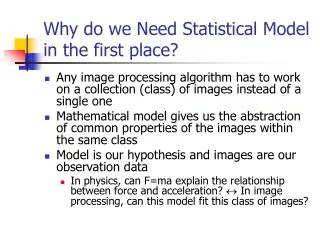
Why do we Need Statistical Model in the first place?
350 likes | 468 Views
Statistical models are crucial in image processing as they enable algorithms to work on collections of images rather than isolated ones. These models abstract meaningful properties from datasets, helping us understand relationships within the data, such as correlation and dependency. In applications like texture synthesis and image denoising, statistical modeling aids in evaluating performance, ensuring generated samples resemble observed data. Furthermore, challenges such as the curse of dimensionality and the need for methods like autoregressive models highlight the complexity of statistical modeling in high-dimensional spaces.

Why do we Need Statistical Model in the first place?
E N D
Presentation Transcript
Why do we Need Statistical Model in the first place? • Any image processing algorithm has to work on a collection (class) of images instead of a single one • Mathematical model gives us the abstraction of common properties of the images within the same class • Model is our hypothesis and images are our observation data • In physics, can F=ma explain the relationship between force and acceleration? In image processing, can this model fit this class of images?
Introduction to Texture Synthesis • Motivating applications • Texture synthesis vs. image denoising • Statistical image modeling revisited • Modeling correlation/dependency • Transform-domain texture synthesis • Nonparametric texture synthesis • Performance evaluation issue
What is Image/Texture Model? texture speech Analysis Analysis Pitch, LPC Residues … P(X): parametric /nonparametric Synthesis Synthesis
How do we Tell the Goodness of a Model? • Synthesis (in statistical language, it is called sampling) Does the generated sample (experimental result) look like the data of our interests? Computer simulation Hypothesized model Does the generated sequence (experimental result) contain the same number of Heads and Tails? Flip the coin A fair coin?
Discrete Random Variables (taken from EE465) Example III: For a gray-scale image (L=256), we can use the notation p(rk), k = 0,1,…, L - 1, to denote the histogram of an image with L possible gray levels, rk, k = 0,1,…, L - 1, where p(rk) is the probability of the kth gray level (random event) occurring. The discrete random variables in this case are gray levels. Question: What is wroning with viewing all pixels as being generated from an independent identically distributed (i.i.d.) random variable
To Understand the Problem • Theoretically, if all pixels are indeed i.i.d., then random permutation of pixels should produce another image of the same class (natural images) • Experimentally, we can write a simple MATLAB function to implement and test the impact of random permutation
Random Process • Random process is the foundation for doing research in the field of communication and signal processing (that is why EE513 is the core requirement for qualified exam) • Random processes is the vector generalization of (scalar) random variables
Correlation and Dependency (N=2) If the condition holds, then the two random variables are said to be uncorrelated. From our earlier discussion, we know that if x and y are statistically independent, then p(x, y) = p(x)p(y), in which case we write Thus, we see that if two random variables are statistically independent then they are also uncorrelated. The converse of this statement is not true in general.
Covariance of two Random Variables The moment µ11 is called the covariance of x and y.
Recall: How to Calculate E(XY)? … … X … … Y Empirical solution: Note: When Y=X, we are getting autocorrelation
Stationary Process* N N T T+K space/time location P(X1,…,XN)=P(XK+1,…,XK+N) for any K,N (all statistics is time invariant) order of statistics
Gaussian Process With mean vector m and covariance matrix C For convenience, we often assume zero mean (if it is nonzero mean, we can subtract the mean) For Gaussian process, it is stationary as long as its first and second order statistics are time-invariant The question is: is the distribution of observation data Gaussian or not?
The Curse of Dimensionality • Even for a small-size image such as 64-by-64, we need to model it by a random process in 4096-dimensional space (R4096) whose covariance matrix is sized by 4096-by-4096 • Curse of dimensionality was pointed out by E. Bellman in 1960s; but even computing resource today cannot handle the brute-force search of nearest-neighbor search in relatively high-dimensional space.
Markovian Assumption Pafnuty L. Chebyshev 1821 - 1894 Andrei A. Markov 1856 - 1922 Andrey N. Kolmogorov 1903 - 1987
A Simple Idea The future is determined by the present but is independent of the past Note that stationarity and Markovianity are two “orthogonal” perspectives of imposing constraints to random processes
Markov Process N-th order Markovian N past samples Parametric or non-parametric characterization
Autoregressive (AR) Model Parametric model (Linear Prediction) z-transform An infinite impulse response (IIR) filter
Example: AR(1) r(k) Autocorrelation function k a=0.9
Yule-Walker Equation Covariance C
Wiener Filtering In practice, we do not know autocorrelation functions but only observation data X1,…,XM Approach 1: empirically estimate r(k) from X1,…,XM Approach 2: Formulate the minimization problem of Exercise: you can verify they end up with the same results
Least-Square Estimation M equations, N unknown variables
Least-Square Estimation (Con’d) rx Rxx If you write it out, it is exactly the empirical way of estimating autocorrelation functions – now you have got the third approach
From 1D to 2D 6 2 3 4 4 3 2 1 Xm,n 5 5 1 Xm,n 8 7 6 Causal neighborhood Noncausal neighborhood Causality of neighborhood depends on different applications (e.g., coding vs. synthesis)
Experimental Justifications AR model parameters Analysis original random excitation Synthesis
Failure Example (I) Analysis and Synthesis N=8,M=4096 Another way to look at it: if X and Y are two images of disks, will (X+Y)/2 produce another disk image?
Failure Example (II) Analysis and Synthesis N=8,M=4096 Note that the failure reason of this example is different from the last example (N is not large enough)
Summary for AR Modeling • We start from AR models because they are relatively simple and well understood (not just for images but also for speech coding, stock market prediction …) • AR model parameters are related to the second-order statistics by Yule-Walker equation • AR model is equivalent to IIR filtering (linear prediction decorrelates the input signal)
Improvement over AR Model • Doubly stochastic process* • In stationary Gaussian process, second-order statistics are time/spatial invariance • In doubly stochastic process, second-order statistics (e.g., covariance) are modeled by another random process with hidden variables • Windowing technique • To estimate spatially varying statistics
Why do We need Windows? • Nothing to do with Microsoft • All images have finite dimensions – they can be viewed as the “windowed” version of natural scenes • Any empirical estimation of statistical attributes (e.g., mean, variance) is based on the assumption that all N samples observe the same distribution • However, how do we know this assumption is satisfied?
1D Rectangular Window X(n) n W=(2T+1)
2D Rectangular Window Loosely speaking, parameter estimation from a localized window is a compromised solution to handle spatially varying statistics W=(2T+1) Such idea is common to other types of non-stationary signals too (e.g., short-time speech processing) W=(2T+1)
Example As window slides though the image, we will observe that AR model parameters vary from location to location A B Q: AR coefficients at B and C differ from those at A but for different reasons, Why? C
What is Next? • Apply linear transformations • A detour of wavelet transforms • Wavelet-space statistical models • Application into texture synthesis • From parametric to nonparametric • Patch-based nonparametric models • Texture synthesis examples • Application into image inpainting