Understanding AdaBoost: Enhancing Classification with Sequential Learning
This chapter delves into AdaBoost, a pioneering supervised learning method that enhances weak classifiers by combining them into a strong ensemble through iterative adjustments to data weights. It explains the principles behind boosting, how to construct boosting trees, and the mechanics of AdaBoost, including the sequential application of weak classifiers and the re-weighting of misclassified samples. The discussion includes performance evaluations and comparisons, showcasing boosting's effectiveness in reducing error rates in classification tasks while addressing the challenges and considerations of using decision trees in this context.


Understanding AdaBoost: Enhancing Classification with Sequential Learning
E N D
Presentation Transcript
Chapter 10 Boosting May 6, 2010
Outline • Adaboost • Ensemble point-view of Boosting • Boosting Trees • Supervised Learning Methods
AdaBoost • Freund and Schapire (1997). • Weak classifiers • Error rate only slightly better than random guessing • Applied sequentially to repeatedly modified versions of the data, to produce a sequence {Gm(x) | m = 1,2,…,M} of weak classifiers • Final prediction is a weighted majority vote G(x) = sign( Sm [am Gm(x)] )
Data Modification and Classifier Weightings • Apply weights (w1,w2,…,wN) to each training example (xi,yi), i = 1, 2,…,N • Initial weights wi = 1/N • At step m+1, increase weights of observations misclassified by Gm(x) • Weight each classifier Gm(x) by the log odds of correct prediction on the training data.
Initialize Observation Weights wi = 1/N, i = 1,…,N For m = 1 to M: Fit a classifier Gm(x) to the training data using weights wi Compute Compute Set Output Algorithm for AdaBoost
Simulated Example • X1,…,X10 iid N(0,1) • Y = 1 if S Xj > c210(0.5) = 9.34 = median • Y = -1 otherwise • N = 2000 training observations • 10,000 test cases • Weak classifier is a “stump” • two-terminal-node classification tree • Test set error of stump = 46% • Test set error after boosting = 12.2% • Test set error of full RP tree = 26%
Boosting Fits an Additive Model Model Choice of basis Single Layer Neural Net s(g0 + g1(x)) Wavelets g for location & scale MARS g gives variables & knots Boosted Trees g gives variables & split points
Forward Stagewise Modeling • Initialize f0(x) = 0 • For m = 1 to M: • Compute • Set • Loss: L[y,f(x)] • Linear Regression: [y - f(x)]2 • AdaBoost: exp[-y*f(x)]
Exponential Loss • For exponential loss, the minimization step in forward stage-wise modeling becomes • In the context of a weak learner G, it is • Can be expressed as
Solving Exponential Minimization • For any fixed b > 0, the minimizing Gm is the {-1,1} valued function given by Classifier that minimizes training error loss for the weighted sample. • Plugging in this solution gives
AdaBoost fits an additive model where the basis functions Gm(x) optimize exponential loss stage-wise Population minimizer of exponential loss is the log odds Decision trees don’t have much predictive capability, but make ideal weak/slow learners especially stumps Generalization of Boosting Decision Trees - MART Shrinkage and slow learning Connection between forward stage-wise shrinkage and Lasso/LAR Tools for interpretation Random Forests Insights and Outline
General Properties of Boosting • Training error rate levels off and/or continues to decrease VERY slowly as M grows large. • Test error continues to decrease even after training error levels off • This phenomenon holds for other loss functions as well as exponential loss.
Why Exponential Loss? • Principal virtue is computational • Minimizer of this loss is (1/2) log odds of P(Y=1 | x), • AdaBoost predicts the sign of the average estimates of this. • In the Binomial family (logistic regression), the MLE of P(Y=1 | x) is the solution corresponding to the loss function • Y’ = (Y+1)/2 is the 0-1 coding of output. • This loss function is also called the “deviance.”
Loss Functions and Robustness • Exponential Loss concentrates much more influence on observations with large negative margins y f(x). • Binomial Deviance spreads influence more evenly among all the data • Exponential Loss is especially sensitive to misspecification of class labels • Squared error loss places too little emphasis on points near the boundary • If the goal is class assignment, a monotone decreasing function serves as a better surrogate loss function
Exponential Loss: Boosting Margin Larger margin Penalty over negative range than positive range
Decision trees are not ideal tools for predictive learning Advantages of Boosting improves their accuracy, often dramatically Maintains most of the desirable properties Disadvantages Can be much slower Can become difficult to interpret (if M is large) AdaBoost can lose robustness against overlapping class distributions and mislabeling of training data Boosting Decision Trees
Ensembles of Trees • Boosting (forward selection with exponential loss) • TreeNet/MART (forward selection with robust loss) • Random Forests (trade-off between uncorrelated components [variance] and strength of learners [bias])
Boosting Trees Forward Selection: Note: common loss function L applies to growing individual trees and to assembling different trees.
Random Forests • “Random Forests” grows many classification trees. • To classify a new object from an input vector, put the input vector down each of the trees in the forest. Each tree gives a classification, and we say the tree "votes" for that class. • The forest chooses the classification having the most votes (over all the trees in the forest).
Random Forests • Each tree is grown as follows: • If the number of cases in the training set is N, sample N cases at random - but with replacement, from the original data. This sample will be the training set for growing the tree. • If there are M input variables, a number m<<M is specified such that at each node, m variables are selected at random out of the M and the best split on these m is used to split the node. The value of m is held constant during the forest growing. • Each tree is grown to the largest extent possible. There is no pruning.