Download
1 / 41
440 likes | 649 Views
Mathematical Programming. ECE 665 Professor Maciej Ciesielski By DFG. Overview. Classical optimization deals with unconstrained optimization problems. For the minimization problem: Min f(x) subject to g(x) = 0

E N D
Mathematical Programming ECE 665 Professor Maciej Ciesielski By DFG
Overview • Classical optimization deals with unconstrainedoptimization problems. • For the minimization problem: Min f(x) subject to g(x) = 0 The solution is to move the constraints to the function and solve the unconstrained optimization problem. • Penalty function method: replace f(x) by F(x) = f(x)+ M( g(x))2, M >> 0 • Lagrangian multipliers: replace f(x) by L(x,λ) = f(x) + Σ λi gi(x) At the optimum point, x*, L(x*, λ) = f(x*)
Outline • Mathematical programming paradigm • Feasible solutions? • Convexity • Concave • Concept example • Geometric solution • Fundamental theorem of LP • Simplex • Example • LP Modifications
Mathematical Programming paradigm Mathematical Programming Paradigm A mathematical program is an optimization problem of the form: • Maximize (or Minimize) f(x) subject to: • g(x) = 0 • h(x) ≥ 0 where x = [x1,...xn] is a subset of Rn, the functions g and h are called constraints, and f is called the objective function.
The Nature of Mathematical Programming Of course there are some forms that deviate from this paradigm. Important examples are: • Fuzzy mathematical program • Goal program • Multiple objectives • Randomized program • Stochastic program Therefore it is typically a modeling issue to find an standard form to solve the mathematical programming.
Mathematical Programming Paradigm Min or Max f(x) Subject to: g(x) = 0 h(x) ≥ 0 When is it feasible? A point x is feasible if it is in X and satisfies the constraints: • g(x) = 0 and h(x) ≥ 0. A point x* is optimal if it is feasible and if the value of the objective function is: • For Maximization not less than that of any other feasible solution: f(x*) ≥ f(x) for all feasible x. • For Minimization not greater than that of any other feasible solution: f(x*) ≤ f(x) for all feasible x.
Mathematical Programming Paradigm Min or Max f(x) Subject to: g(x) = 0 h(x) ≥ 0 Convexity • To obtain global optimum, it is important that the constraint set {x | g(x) = 0, h(x) ≥ 0} and the function f(x) be convex. If the functionis convex over a convex constraint set, then local minimun is also a globa1 minimum
Convexity • Set convexity(If any two points are in the set, so is their line segment) Convex set non-convex set • Function convexity Convex function non-convex function ???
Epigraph: region on or above the graph Convexity A function f:X–>R is said to be convex if: • Its epigraph is convex. • X is a convex set, and for x,y X and a[0, 1]: f(ax + (1-a)y) ≤ af(x) + (1-a)f(y)
Convexity If the functionis convex over a convex constraint set, then local minimun is also a globa1 minimum
Hypograph: region below the graph Concave • It is define for maximization, and it is the negative of convexity. • A function f is concave if its hypograph is convex
Concave If the functionis concave over a convex constraint set, then local maximun is also a globa1 maximum
Quadratic Programming Concept Example • Can we minimize based on the local minimum? f(x) = xTQx • Subject to: Ax ≥ b x ≥ 0 • Where Q is an n x n symmetric matrix, A is a constraint matrix, and b is a constraint vector.
Concept Example • If xTQx > 0 for every x 0. The matrix Q is positive definite. In which case its eigenvalues are non-negative, and the quadratic form is a convex function. Thus f is convex. As Q is a symmetric matrix, these eingenvalues will be reals. • Ax ≥ b defines a convex constraint set, as its solution is a Rk space. (A convex polyhedron) • f and the constraint set are convex, therefore, finding the local minimum also finds the global minimum.
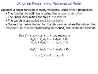
Linear Programming (LP) • The goal of Linear programming is to: (Max)Minimize: CTx Subject to: Ax ≥ b x ≥ 0 Where CT is a coefficient vector for f, A is a constraint matrix, and b es a constraint vector. • The constraint set: {x | Ax ≥ b} is a convex polyhedron, and f is linear so it is convex. Therefore, LP has convexity, and the local min/max is the global min/max
LP Example (Problem Enunciation) Optimization problem: • 2 types of products are made by the factory • 3 machines are needed to make each productConstraints: Machines are available for a limited time during one production session: • time on A ≤50 hours • time on B ≤35 hours • time on C ≤ 80 hours
LP Example (Problem Enunciation) To complete the product, each lot must be processed by all three machines for a certain number of hours Required manufacturing time Machines A B C 1 Products 2 Time Constraint: 50 35 80
LP Example (Problem Enunciation) Profit: • Product 1 can be sold for $100 per lot • Product 2 can be sold for $80 per lot Optimization Problem: • Design the production schedule which maximizes the profit of both products manufactured during one production session.
LP Example (Problem Formulation) • Formulation x1 = number of lots of product 1 x2 = number of lots of product 2 max f (x) = 100x1 + 80x2 10x1 + 5x2 ≤ 50 5x1 + 5x2 ≤ 35 5x1 + 15x2 ≤ 80
F(x) = 800 Sol: X1 = 3 X2 = 4 LP Example (Geometric Solution) x2 • Geometric solution: Family of curves, constant for x1, x2 F(x) = 100 x1 +80 x2 =800 (const) (a) 10x1 +5x2 50 (b) 5x1 + 5x2 35(c) 5x1 + 15x2 80 10 5 4 P2 Extreme point P1 x1 P0 c 3 5 10 15 a b
LP Example (Standard Linear Program Approach) • Convert the problem to a standard Linear Program (LP): Max f(x) = 100x1+ 8Ox2 + 0s1 + 0s2 + 0s3 10x1+ 5x2 + s1 = 50 Subject to: 5x1 + 5x2 + s2 = 35 5x1+ 15x2+ s3 = 80 Basis New Matrix A Why the Basis??
Basis and Basic solution Why the Basis? • Because it finds a basic solution Given a system of equalities: Ax = b where: x = n-vector, b = m-vector, A = mn matrix select a set of m linearly independent columns such that (mm) matrix B is nonsingular, i.e. |B| 0. Then one may uniquely solve the equation: Bxb= b where: xbis an m-element subvector of x. Max f(x) = 100x1+ 8Ox2 + 0s1 + 0s2 + 0s3 Subject to: 10x1+ 5x2 + s1 = 50 5x1 + 5x2 + s2 = 35 5x1+ 15x2 + s3 = 80
Basis and Basic solution By putting x=(xb,0) we obtain a solution to Ax = b Such a solution (with n-m components of xnot associated with columns of Bmm)to theresulting set of equations is said to be a basic solution with regard to the basis B. The Xbvariables, associated with columns of B, are called basic variables. Basic Feasible Solution If a feasible solution (i.e. the one which satisfies all contraints) is also basic, it is called a basic feasible solution. Max f(x) = 100x1+ 8Ox2 + 0s1 + 0s2 + 0s3 Subject to: 10x1+ 5x2 + s1 = 50 5x1 + 5x2 + s2 = 35 5x1+ 15x2 + s3 = 80 basic variables B.F.S x1 = 0 s1 = 50 s3 = 80 x2 = 0 s2 = 35
Fundamental Theorem of Linear Programming Given an LP in standard form min CTx subject to Ax = b x 0 where A is mn matrix of rank m (i.e. m < n and the m rows are linear independent), • If there is a feasible solution, there is a basic feasible solution • If there is an optimal feasible solution, there is an optimal basic feasible solution
Fundamental Theorem of Linear Programming This theorem shows that it is necessary only to consider basic feasible solutions when seeking an optimal solution to a linear program, as the optimal value is always achieved as such a solution Ultimate goal: • find a basic feasible solution with a base B composed of original variables only, and which is optimum.
LP Example (Basic Feasible solution) ƒ (x) = 100 x1 +80 x2 +0 s1 +0 s2 +0 s3 • Solution: x1 = 0, x2 = 0, s1 = 50, s2 = 35, s3 = 80, is a basic feasible solution: point P0(0,0) Extreme point • Function value:F(0, 0, 50, 35, 80) = 0 basis
LP Example (Basic Feasible solution) x2 The basic feasible solution in the Geometric approach is in the Extreme Point. 10 5 4 P2 Extreme point P1 x1 P0 c 3 5 10 15 a b
Simplex Method • Proceed from one basic feasible solution (extreme point) to another, in such a way as to continually decrease /increase the value of the f (x) until a minimum / maximum is reached. General comments: • It is easy find initial basic feasible solutions with slack variables. • Finding initial basic solution is part of the Simplex method (Lue 84).
Simplex Algorithm • Select the column, such that the new resulting basic feasible solution will yield a lower /greater valueto f(x) than the previous one. • Select the pivot element in that column. By an elementary evaluation determine: • Which vector ajshould enter the basis (so that f(x) is reduced), and • Which vector should leave the basis.
Simplex Algorithm Construct a Simplex Table, [A, b ] appended by a row at the top with cost coefficients and current cost. Point P0 (0,0) F(0,0,50,35,80) = 0
Simplex Algorithm • Step 1. Select column q with rq > 0. (xqenters the basis) q : rq = max ri • Step 2. Select row p, which defines pivot element p in column q Which minimizes ratio: p : = min for positive yiq i
Simplex Algorithm • Step 3. Pivot on element ypq and update the table (update all rows, including the top one) • In row p divide ypj by ypq , j = 0, 1,…, n • Subtract from each row i p ypj , j = 0, 1,…, n
Step2: min of Step1: max rq Therfore: ypq = 10 Simplex Algorithm Example • Pivot on y11 Point P0 (0,0) F(0,0,50,35,80) = 0
Step 3.B: in row i ≠ p Step 3.A: in row p Simplex Algorithm Example • Update table Point P0 (0,0) F(0,0,50,35,80) = 0 Point P1 (5,0) F(5,0,0,10,55) = 500
Step2: min of Step1: max rq Therfore: ypq = 4 Simplex Algorithm Example • Pivot on y22 Point P1 (5,0) F(5,0,0,10,55) = 500
Step 3.B: in row i ≠ p Step 3.A: in row p Simplex Algorithm Example • Update table Point P1 (5,0) F(5,0,0,10,55) = 500 Point P2 (3,4) F(3,4,0,0,5) = 620
Step1: all rq< 0 Terminate algorithm Sol: X1 = 3 X2 = 4 Simplex Algorithm Example • Pivot on Point P2 (3,4) F(3,4,0,0,5) = 620
Linear Programming Modifications 1. Maximization max c t x = min (-c t x) 2. Unconstrained x let x = x+ - x -; x+, x - 0) min (c t x+ - c t x -) x+ x - s. to [A, -A] = b x+, x - 0
Linear Programming Modifications 3. Constraint set:Ax b Slack variables,xs : Ax + xs = b x xs [A, I ] = b x xs min [cT , 0] x , xs 0 Columns corresponding to xsform a basic solution
Linear Programming Modifications 4. Constraint set:Ax ≥ b Surplus variables,xp : Ax - xp = b x xp [A, -I ] = b x xp min [cT , 0] x , xp 0
Linear Programming Modifications 5. Artificial variables, xa: Ax - xp + xa = b (cannot star with negative basis of xp ) x xp xa min [cT , 0 , k I ] x xp xa [A, -I , I ] = b S. to x , xp ,xa 0 Columns corresponding to xaform a basic solution