Image Enhancement in Frequency Domain
170 likes | 846 Views
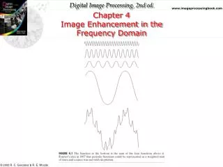
Image Enhancement in Frequency Domain. Image and Its Fourier Spectrum. Basic Steps Multiply pixel f(x,y) of the input image by (-1) x+y . Compute F(u,v), the DFT G(u,v)=F(u,v)H(u,v) g1(x,y)=F -1 {G(u,v)} g(x,y) = g1(x,y)*(-1) x+y. Filtering in Frequency Domain: Basic Steps. Notch Filter.

Image Enhancement in Frequency Domain
E N D
Presentation Transcript
Basic Steps Multiply pixel f(x,y) of the input image by (-1)x+y. Compute F(u,v), the DFT G(u,v)=F(u,v)H(u,v) g1(x,y)=F-1{G(u,v)} g(x,y) = g1(x,y)*(-1)x+y Filtering in Frequency Domain: Basic Steps
Notch Filter • The frequency response F(u,v) has a notch at origin (u = v = 0). • Effect: reduce mean value. • After post-processing where gray level is scaled, the mean value of the displayed image is no longer 0.
Fourier Transform pair of Gaussian function Depicted in figures are low-pass and high-pass Gaussian filters, and their spatial response, as well as FIR masking filter approximation. High pass Gaussian filter can be constructed from the difference of two Gaussian low pass filters. Gaussian Filters
D(u,v): distance from the origin of Fourier transform Gaussian Low Pass Filters
The cut-off frequency Do determines % power are filtered out. Image power as a function of distance from the origin of DFT (5, 15, 30, 80, 230) Ideal Low Pass Filters
Blurring can be modeled as the convolution of a high resolution (original) image with a low pass filter. Effects of Ideal Low Pass Filters
Ideal high pass filter Butterworth high pass filter Gaussian high pass filter High Pass Filters
Ideal HPF Do = 15, 30, 80 Butterworth HPF n = 2, Do = 15, 30, 80 Gaussian HPF Do = 15, 30, 80 Applications of HPFs
3D plots of the Laplacian operator, its 2D images, spatial domain response with center magnified, and Compared to the FIR mask approximation Laplacian HPF