A small case study
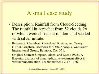
A small case study. Description: Rainfall from Cloud-Seeding. The rainfall in acre-feet from 52 clouds 26 of which were chosen at random and seeded with silver nitrate.

A small case study
E N D
Presentation Transcript
A small case study • Description: Rainfall from Cloud-Seeding. The rainfall in acre-feet from 52 clouds 26 of which were chosen at random and seeded with silver nitrate. • Reference: Chambers, Cleveland, Kleiner, and Tukey. (1983). Graphical Methods for Data Analysis. Wadsworth International Group, Belmont, CA, 351. • Original Source: Simpson, Alsen, and Eden.(1975). A Bayesian analysis of a multiplicative treatment effect in weather modification. Technometrics 17, 161-166. Statistical Data Analysis - Lecture 05 12/03/03
Number of cases: 26 Variable Names: • Unseeded: Amount of rainfall from unseeded clouds (in acre-feet) • Seeded: Amount of rainfall from seeded clouds with silver nitrate (in acre-feet) Statistical Data Analysis - Lecture 05 12/03/03
Step 1: Visually inspect the data • It is easier to look at the order statistics sort the data. First let’s make the data easier to work with clouds<-data.frame(seed=Seeded, u.seed=Unseeded) attach(clouds) Now sort the data. Type: seed<-sort(seed) u.seed<-sort(u.seed) Type clouds to display the data Statistical Data Analysis - Lecture 05 12/03/03
Visual inspection of the data • There are some very large values • There are some very small values • The data does not increase linearly • The data sets look as though they increase at the same rate but there is a shift in mean Statistical Data Analysis - Lecture 05 12/03/03
Plot the data • A histogram of each data set would be helpful • Type: par(mfrow=c(2,1)) # this sets the graph screen # to 2 rows 1 column hist(u.seed) hist(seed) Statistical Data Analysis - Lecture 05 12/03/03
Interpret the histograms • Note the histograms don’t have the same scales so it makes them difficult to compare • Each histogram has a long tail to the right so the data sets are right skewed. • Confirm this by calculating a symmetry statistic for each. • Type: s(seed) s(u.seed) Note the 0.1 – this means we’re using the 0.1 quantile and the 0.9 quantile to calculate the symmetry statistic Statistical Data Analysis - Lecture 05 12/03/03
Get summary statistics • Type: summary(seed) summary(u.seed) • This gives you a five number summary (Min, LQ, Med, UQ, Max) plus the mean • To get the standard deviations type sd(seed) sd(u.seed) • To get the skewness statistics type skewness(seed) skewness(u.seed) Statistical Data Analysis - Lecture 05 12/03/03
Descriptive statistics • Note that the skewness statistic confirms our histogram interpretation and our symmetry statistic. • We can plot the mean and median on each histogram: hist(seed) abline(v=median(seed),col=“red”,lwd=2) abline(v=mean(seed),col=“blue”,lwd=2) hist(u.seed) abline(v=median(u.seed),col=“red”,lwd=2) abline(v=mean(u.seed),col=“blue”,lwd=2) Notice how the median lines up with the centre of the data much better than the mean. • If we want to compare groups it is going to be easier if we transform the data Statistical Data Analysis - Lecture 05 12/03/03
Transforming the data • Choose a sensible transformation either using the sympowerplot function, e.g. sympowerplot(u.seed) sympowerplot(seed) • Or by using the Box-Cox method. bcp(u.seed) bcp(seed) Statistical Data Analysis - Lecture 05 12/03/03
Transforming the data • Box-Cox recommends p = 0.047 and p = 0.118 – therefore a log transformation might work well. If you’re willing to wait awhile try • bcp.bounds(seed) and bcp.bounds(u.seed) • These will give approximate 95% confidence intervals on the powers and they both include 0 • Symmetry power plots recommend p =– 0.1 and p = 0.16 for unseeded and seeded respectively. • Log is easiest to explain, so try that. • Look at log transformed histograms • Still lumpy, but skewness has been reduced Statistical Data Analysis - Lecture 05 12/03/03
Compare the data • Boxplot the transformed data • Join the data into one vector rainfall<-c(log.u.seed, log.seed) • Use the rep command to make a vector of labels corresponding to the unseeded and seeded data gp<-rep(c(“Unseeded”,”Seeded”),c(26,26)) boxplot(split(rainfall,gp)) • QQ-Plot the data qqplot(log.u.seed,log.seed) qq.plot(log.u.seed,log.seed) Statistical Data Analysis - Lecture 05 12/03/03
Compare the data • QQ-plot shows linear trend logged data are from similar distributions • Slope is approximately equal to 1 similar spread • Is the difference in the means significant ? • Two-sample t-test Statistical Data Analysis - Lecture 05 12/03/03
Assumptions of the two samplet-test • The data sets are statistically independent • The data are normally distributed • The data have the same variance • This last assumption can be relaxed if we use Welch’s modification to the t-test Statistical Data Analysis - Lecture 05 12/03/03
Two sample t-test • Control group (unseeded) and treatment group (seeded) were independently measured so data are independent • Log data are approximately unimodal and symmetric, so normality is okay • Check with norplots • Use t.test(log.u.seed,log.seed) Statistical Data Analysis - Lecture 05 12/03/03
Interpret results • 0.01< P <0.05 difference significant at 5% level • 95% C.I does not contain zero difference significant at 5% level • “Based on the data there is evidence to suggest that we reject the null hypothesis (of no difference)” • What does this mean? Statistical Data Analysis - Lecture 05 12/03/03
Interpret the results • We have a 95% c.i. for the difference in the logged means. What does this tell us in terms of the original data? • Not much on this scale – transform estimated difference and c.i. back to original scale Statistical Data Analysis - Lecture 05 12/03/03
Interpret the results • So now we have three numbers 3.14, 1.27 and 7.74 – what do we do with them • “The average amount of rainfall (in acre-feet) is approximately 3 times higher if the clouds are seeded with silver nitrate than if they’re not.” • “With 95% confidence we can say this figure could be as low as 1.3 times or as high as 7.7 times.” Statistical Data Analysis - Lecture 05 12/03/03