Download
1 / 49
490 likes | 681 Views
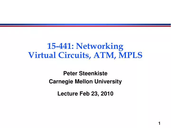
15-441: Networking Virtual Circuits, ATM, MPLS. Peter Steenkiste Carnegie Mellon University Lecture Feb 23, 2010. Outline. Circuit switching refresher Virtual Circuits - general Why virtual circuits? How virtual circuits? -- tag switching! Two modern implementations

E N D
15-441: NetworkingVirtual Circuits, ATM, MPLS Peter Steenkiste Carnegie Mellon UniversityLecture Feb 23, 2010
Outline • Circuit switching refresher • Virtual Circuits - general • Why virtual circuits? • How virtual circuits? -- tag switching! • Two modern implementations • ATM - teleco-style virtual circuits • MPLS - IP-style virtual circuits
Packet Switching • Source sends information as self-contained packets that have an address. • Source may have to break up single message in multiple • Each packet travels independently to the destination host. • Routers and switches use the address in the packet to determine how to forward the packets • Destination recreates the message. • Analogy: a letter in surface mail.
Circuit Switching • Source first establishes a connection (circuit) to the destination. • Each router or switch along the way may reserve some bandwidth for the data flow • Source sends the data over the circuit. • No need to include the destination address with the data since the routers know the path • The connection is torn down. • Example: telephone network.
Circuit Switching Discussion • Traditional circuits: on each hop, the circuit has a dedicated wire or slice of bandwidth. • Physical connection - clearly no need to include addresses with the data • Advantages, relative to packet switching: • Implies guaranteed bandwidth, predictable performance • Simple switch design: only remembers connection information, no longest-prefix destination address look up • Disadvantages: • Inefficient for bursty traffic (wastes bandwidth) • Delay associated with establishing a circuit • Can we get the advantages without (all) the disadvantages?
Virtual Circuits • Each wire carries many “virtual” circuits. • Forwarding based on virtual circuit (VC) identifier • IP header: src, dst, etc. • Virtual circuit header: just “VC” • A path through the network is determined for each VC when the VC is established • Use statistical multiplexing for efficiency • Can support wide range of quality of service. • No guarantees: best effort service • Weak guarantees: delay < 300 msec, … • Strong guarantees: e.g. equivalent of physical circuit
Packet Switching andVirtual Circuits: Similarities • “Store and forward” communication based on an address. • Address is either the destination address or a VC identifier • Must have buffer space to temporarily store packets. • E.g. multiple packets for some destination arrive simultaneously • Multiplexing on a link is similar to time sharing. • No reservations: multiplexing is statistical, i.e. packets are interleaved without a fixed pattern • Reservations: some flows are guaranteed to get a certain number of “slots” D B C B A A
Virtual Circuits Versus Packet Switching • Circuit switching: • Uses short connection identifiers to forward packets • Switches know about the connections so they can more easily implement features such as quality of service • Virtual circuits form basis for traffic engineering: VC identifies long-lived stream of data that can be scheduled • Packet switching: • Use full destination addresses for forwarding packets • Can send data right away: no need to establish a connection first • Switches are stateless: easier to recover from failures • Adding QoS is hard • Traffic engineering is hard: too many packets!
Circuit Switching Switch Input Ports Output Ports Connects (electrons, light, or bits) ports to ports
Packet switched vs. VC VCI Dst Payload Payload R1 packet forwarding table: Dst R2 1 3 A R2 2 1 3 4 1 3 R1 R4 Dst 2 4 2 4 1 3 B R3 2 4 Different paths to same destination! (useful for traffic engineering!) R1 VC table: VC 1 R2 VC 2 R3
Virtual Circuit VCI Payload Payload 1 3 A R2 2 1 3 4 1 3 R1 R4 Dst 2 4 2 4 1 3 B R3 2 4 Challenges: - How to set up path? - How to assign IDs?? R1 VC table: VC 5 R2 R2 VC table: VC 5 R4
Connections and Signaling • Permanent vs. switched virtual connections (PVCs, SVCs) • static vs. dynamic. PVCs last “a long time” • E.g., connect two bank locations with a PVC • SVCs are more like a phone call • PVCs administratively configured (but not “manually”) • SVCs dynamically set up on a “per-call” basis • Topology • point to point • point to multipoint • multipoint to multipoint • Challenges: How to configure these things? • What VCI to use? • Setting up the path
Virtual Circuit Switching:Label (“tag”) Swapping 1 3 A R2 2 1 3 4 • Global VC ID allocation -- ICK! Solution: Per-link uniqueness. Change VCI each hop. Input Port Input VCI Output Port Output VCI R1: 1 5 3 9 R2: 2 9 4 2 R4: 1 2 3 5 1 3 R1 R4 Dst 2 4 2 4 1 3 B R3 2 4
Label (“tag”) Swapping • Result: Signalling protocol must only find per-link unused VCIs. • “Link-local scope” • Connection setup can proceed hop-by-hop. • Good news for our setup protocols!
PVC connection setup • Manual? • Configure each switch by hand. Ugh. • Dedicated signalling protocol • E.g., what ATM uses • Piggyback on routing protocols • Used in MPLS. E.g., use BGP to set up
SVC Connection Setup calling party network called party SETUP SETUP CONNECT CONNECT CONNECT ACK CONNECT ACK
Virtual Circuits In Practice • ATM: Teleco approach • Kitchen sink. Based on voice, support file transfer, video, etc., etc. • Intended as IP replacement. That didn’t happen. :) • Today: Underlying network protocol in many teleco networks. E.g., DSL speaks ATM. IP over ATM in some cases. • MPLS: The “IP Heads” answer to ATM • Stole good ideas from ATM • Integrates well with IP • Today: Used inside some networks to provide VPN support, traffic engineering, simplify core. • Other nets just run IP. • Older tech: Frame Relay • Only provided PVCs. Used for quasi-dedicated 56k/T1 links between offices, etc. Slower, less flexible than ATM.
Asynchronous Transfer Mode: ATM • Connection-oriented, packet-switched • (e.g., virtual circuits). • Teleco-driven. Goals: • Handle voice, data, multimedia • Support both PVCs and SVCs • Replace IP. (didn’t happen…) • Important feature: Cell switching
Cell Switching • Small, fixed-size cells [Fixed-length data][header] • Why? • Efficiency: All packets the same • Easier hardware parallelism, implementation • Switching efficiency: • Lookups are easy -- table index. • Result: Very high cell switching rates. • Initial ATM was 155Mbit/s. Ethernet was 10Mbit/s at the same time. (!) • How do you pick the cell size?
ATM Features • Fixed size cells (53 bytes). • Why 53? • Virtual circuit technology using hierarchical virtual circuits (VP,VC). • PHY (physical layer) processing delineates cells by frame structure, cell header error check. • Support for multiple traffic classes by adaptation layer. • E.g. voice channels, data traffic • Elaborate signaling stack. • Backwards compatible with respect to the telephone standards • Standards defined by ATM Forum. • Organization of manufacturers, providers, users
Why 53 Bytes? • Small cells favored by voice applications • delays of more than about 10 ms require echo cancellation • each payload byte consumes 125 s (8000 samples/sec) • Large cells favored by data applications • Five bytes of each cell are overhead • France favored 32 bytes • 32 bytes = 4 ms packetization delay. • France is 3 ms wide. • Wouldn’t need echo cancellers! • USA, Australia favored 64 bytes • 64 bytes = 8 ms • USA is 16 ms wide • Needed echo cancellers anyway, wanted less overhead • Compromise
1 2 3 4 5 synchronous asynchronous constant variable bit rate connection-oriented connectionless ATM Adaptation Layers • AAL 1: audio, uncompressed video • AAL 2: compressed video • AAL 3: long term connections • AAL 4/5: data traffic • AAL5 is most relevant to us…
AAL5 Adaptation Layer data pad ctl len CRC . . . ATM header payload (48 bytes) includes EOF flag Pertinent part: Packets are spread across multiple ATM cells. Each packet is delimited by EOF flag in cell.
ATM Packet Shredder Effect • Cell loss results in packet loss. • Cell from middle of packet: lost packet • EOF cell: lost two packets • Just like consequence of IP fragmentation, but VERY small fragments! • Even low cell loss rate can result in high packet loss rate. • E.g. 0.2% cell loss -> 2 % packet loss • Disaster for TCP • Solution: drop remainder of the packet, i.e. until EOF cell. • Helps a lot: dropping useless cells reduces bandwidth and lowers the chance of later cell drops • Slight violation of layers • Discovered after early deployment experience with IP over ATM.
ATM Traffic Classes • Constant Bit Rate (CBR) and Variable Bit Rate (VBR). • Guaranteed traffic classes for different traffic types. • Unspecified Bit Rate (UBR). • Pure best effort with no help from the network • Available Bit Rate (ABR). • Best effort, but network provides support for congestion control and fairness • Congestion control is based on explicit congestion notification • Binary or multi-valued feedback • Fairness is based on Max-Min Fair Sharing. (small demands are satisfied, unsatisfied demands share equally)
IP over ATM • When sending IP packets over an ATM network, set up a VC to destination. • ATM network can be end to end, or just a partial path • ATM is just another link layer • Virtual connections can be cached. • After a packet has been sent, the VC is maintained so that later packets can be forwarded immediately • VCs eventually times out • Properties. • Overhead of setting up VCs (delay for first packet) • Complexity of managing a pool of VCs • Flexible bandwidth management • Can use ATM QoS support for individual connections (with appropriate signaling support)
IP over ATMPermanent VCs • Establish a set of “ATM pipes” that defines connectivity between routers. • Routers simply forward packets through the pipes. • Each statically configured VC looks like a link • Properties. • Some ATM benefits are lost (per flow QoS) • Flexible but static bandwidth management • No set up overheads
ATM Discussion • At one point, ATM was viewed as a replacement for IP. • Could carry both traditional telephone traffic (CBR circuits) and other traffic (data, VBR) • Better than IP, since it supports QoS • Complex technology. • Switching core is fairly simple, but • Support for different traffic classes • Signaling software is very complex • Technology did not match people’s experience with IP • deploying ATM in LAN is complex (e.g. broadcast) • supporting connection-less service model on connection-based technology • With IP over ATM, a lot of functionality is replicated • Currently used as a datalink layer supporting IP.
IP Switching • How to use ATM hardware without the software. • ATM switches are very fast data switches • software adds overhead, cost • The idea is to identify flows at the IP level and to create specific VCs to support these flows. • flows are identified on the fly by monitoring traffic • flow classification can use addresses, protocol types, ... • can distinguish based on destination, protocol, QoS • Once established, data belonging to the flow bypasses level 3 routing. • never leaves the ATM switch • Interoperates fine with “regular” IP routers. • detects and collaborates with neighboring IP switches
IP Switching Example IP IP IP ATM ATM ATM
IP Switching Example IP IP IP ATM ATM ATM
IP Switching Example IP IP IP ATM ATM ATM
IP IP IP IP IP IP IP IP ATM ATM ATM ATM ATM ATM ATM ATM Another View IP IP IP IP
IP SwitchingDiscussion • IP switching selectively optimizes the forwarding of specific flows. • Offloads work from the IP router, so for a given size router, a less powerful forwarding engine can be used • Can fall back on traditional IP forwarding if there are failures • IP switching couples a router with an ATM switching using the GSMP protocol. • General Switch Management Protocol • IP switching can be used for flows with different granularity. • Flows belonging to an application .. Organization • Controlled by the classifier
Multi Protocol Label Switching - MPLS • Selective combination of VCs + IP • Today: MPLS useful for traffic engineering, reducing core complexity, and VPNs • Core idea: Layer 2 carries VC label • Could be ATM (which has its own tag) • Could be a “shim” on top of Ethernet/etc.: • Existing routers could act as MPLS switches just by examining that shim -- no radical re-design. Gets flexibility benefits, though not cell switching advantages Layer 3 (IP) header Layer 3 (IP) header MPLS label Layer 2 header Layer 2 header
MPLS + IP • Map packet onto Forward Equivalence Class (FEC) • Simple case: longest prefix match of destination address • More complex if QoS of policy routing is used • In MPLS, a label is associated with the packet when it enters the network and forwarding is based on the label in the network core. • Label is swapped (as ATM VCIs) • Potential advantages. • Packet forwarding can be faster • Routing can be based on ingress router and port • Can use more complex routing decisions • Can force packets to followed a pinned route
MPLS core, IP interface MPLS tag assigned MPLS tag stripped IP IP IP IP C 1 3 A R2 2 1 3 4 1 3 R1 R4 2 4 2 4 1 3 B R3 D 2 4 MPLS forwarding in core
MPLS use case #1: VPNs 10.1.0.0/24 10.1.0.0/24 C 1 3 A R2 2 1 3 4 1 3 R1 R4 2 4 2 4 1 3 B R3 D 2 4 10.1.0.0/24 10.1.0.0/24 MPLS tags can differentiate green VPN from orange VPN.
MPLS use case #2: Reduced State Core EBGP EBGP C A R2 A-> C pkt Internal routers must know all C destinations R1 R4 IP Core R3 EBGP C 1 3 A R2 2 1 3 4 1 3 R1 MPLS Core R4 2 4 2 4 R1 uses MPLS tunnel to R4. R1 and R4 know routes, but R2 and R3 don’t. 1 3 R3 2 4 .
MPLS use case #3: Traffic Engineering • As discussed earlier -- can pick routes based upon more than just destination • Used in practice by many ISPs, though certainly not all.
MPLS Mechanisms • MPLS packet forwarding: implementation of the label is technology specific. • Could be ATM VCI or a short extra “MPLS” header • Supports stacked labels. • Operations can be “swap” (normal label swapping), “push” and “pop” labels. • VERY flexible! Like creating tunnels, but much simpler -- only adds a small label. Label CoS S TTL 8 20 3 1
MPLS Discussion • Original motivation. • Fast packet forwarding: • Use of ATM hardware • Avoid complex “longest prefix” route lookup • Limitations of routing table sizes • Quality of service • Currently mostly used for traffic engineering and network management. • LSPs can be thought of as “programmable links” that can be set up under software control • on top of a simple, static hardware infrastructure
Take Home Points • Costs/benefits/goals of virtual circuits • Cell switching (ATM) • Fixed-size pkts: Fast hardware • Packet size picked for low voice jitter. Understand trade-offs. • Beware packet shredder effect (drop entire pkt) • Tag/label swapping • Basis for most VCs. • Makes label assignment link-local. Understand mechanism. • MPLS - IP meets virtual circuits • MPLS tunnels used for VPNs, traffic engineering, reduced core routing table sizes
--- Extra Slides --- Extra information if you’re curious.
LAN Emulation • Motivation: making a non-broadcast technology work as a LAN. • Focus on 802.x environments • Approach: reuse the existing interfaces, but adapt implementation to ATM. • MAC - ATM mapping • multicast and broadcast • bridging • ARP • Example: Address Resolution “Protocol” uses an ARP server instead of relying on broadcast.
Further reading - MPLS • MPLS isn’t in the book - sorry. Juniper has a few good presentations at NANOG (the North American Network Operators Group; a big collection of ISPs): • http://www.nanog.org/mtg-0310/minei.html • http://www.nanog.org/mtg-0402/minei.html • Practical and realistic view of what people are doing _today_ with MPLS.
An AlternativeTag Switching • Instead of monitoring traffic to identify flows to optimize, use routing information to guide the creation of “switched” paths. • Switched paths are set up as a side effect of filling in forwarding tables • Generalize to other types of hardware. • Also introduced stackable tags. • Made it possible to temporarily merge flows and to demultiplex them without doing an IP route lookup • Requires variable size field for tag A C A A B B B C
IP Switchingversus Tag Switching • Flows versus routes. • tags explicitly cover groups of routes • tag bindings set up as part of route establishment • flows in IP switching are driven by traffic and detected by “filters” • Supports both fine grain application flows and coarser grain flow groups • Stackable tags. • provides more flexibility • Generality • IP switching focuses on ATM • not clear that this is a fundamental difference
Packets over SONET • Same as statically configured ATM pipes, but pipes are SONET channels. • Properties. • Bandwidth management is much less flexible • Much lower transmission overhead (no ATM headers) mux OC-48 mux mux