3.SED Fitting Method
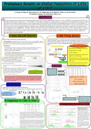
3.SED Fitting Method. Salpeter IMF (1955) + Star Formation History + Metallicity. Stellar evolutionary track (Padova 1994). Model Spectrum. Shift redward to z=4.8, Calzetti extinction law(2000). Observed SEDs. Model SED. Convolve with filter response function.

3.SED Fitting Method
E N D
Presentation Transcript
3.SED Fitting Method Salpeter IMF (1955) + Star Formation History + Metallicity Stellar evolutionary track (Padova 1994) Model Spectrum Shift redward to z=4.8, Calzetti extinction law(2000) Observed SEDs Model SED Convolve with filter response function Best fitted model with known population (i.e. stellar mass, age, E(B-V), SFR) Minimization method: GOODS-N GOODS-FF Stellar masses: Mʘ Age: 1-550 Myr E(B-V): 0.00-0.58 mag SFR: 20-3400 Mʘ/yr B V R NB711 Ic z’ 33 objects are picked up as LAE candidates at z=4.8. Figure3. A plot between IRAC ch2 magnitudes (4.5m) against derived stellar masses indicating the relation of the stellar mass and rest-frame optical magnitudes. Figure2. A plot of IRAC ch1 magnitude (3.6m) vs the star formation rates (SFR) Preliminary Results on Stellar Populations of LAEs at z=4.8 S. Yuma, K. Ohta, K. Yabe (Kyoto U.), K. Shimasaku, M. Yoshida (U. Tokyo), I. Iwata (OAO), M. Ouchi (Carnegie), M. Sawicki (St. Mary’s U.) ABSTRACT We present the preliminary Spectral Energy Distribution (SED) fitting results of Lyman Alpha Emitters (LAEs) at z=4.8 in GOODS-N and its flanking fields. Observing through the NB711 narrow-band filter [ Å, FWHM = 73 Å] attached on Suprime-Cam, Subaru telescope, we obtained 33 Lyman Alpha Emitters (LAEs). 8 of them are detected in mid-IR data obtained by IRAC camera on Spitzer Space Telescope (SST) toward GOODS-N and flanking field. The rest-frame UV to optical SEDs of 8 LAEs at z=4.8 are constructed. After fitting the observed SEDs with stellar population synthesis models by Bruzual & Charlot(2003), various physical properties of LAEs are derived. In this work, we adopt the constant star formation history with fixed 0.2Zʘ metallicity. By taking into account the H emission line, the best fitted stellar mass and age are in the ranges of Mʘ and 1-550 Myr, respectively. These values are broadly consistent with other studies on LAEs at other redshifts (e.g. Gawiser et al.2006&2007, Lai et al.2007, Nilsson et al.2007, Finkelstein et al.2007, and Pirzkal et al.2007). However, our derived star formation rates (SFRs) and dust extinctions are significantly larger than those of LAEs by other studies. Comparing the derived mass and age with those of LBGs at z~5, it is found that our LAE candidates are younger and less massive than LBGs. 1.Data and LAE Selection Broadband photometry of 8 objects are used to construct Spectral Energy Distributions (SEDs). The SEDs consist of photometry from 4 bandpasses which are Ic and z’ bands from Subaru data and IRAC channels 1 and 2. The observed SEDs are then fitted with population synthesis models by Bruzual&Charlot (2003) as shown in the diagram below: • Data: From Ground-base to space telescope • The optical data are obtained by Suprime-Cam on Subaru Telescope using NB711 narrow band and BVRIcz’ broadbands centering at Hubble Deep Field-North [RA(2000)= , Dec(2000)= ]. The observations are operated in 2005 April. • Mid-IR data • GOODS-N field : There are publicly available data taken under SST Legacy Science Program by IRAC camera on Spitzer Space Telescope (SST) in 4 bandpasses. [http://ssc.spitzer.caltech.edu/legacy/] • GOODS-FF: The flanking regions are also observed by using the same instrument (i.e. IRAC on SST) in 2005 December and 2006 June. Note that the data observed by us are ~1 mag shallower than those in GOODS-N field. Parameters used to build models: • BC03 Padova evolutionary track(1994) • Salpeter IMF 0.1-100 Mʘ • 0.2Zʘ metallicity • Calzetti dust extinction law (2000) with E(B-V) = 0-1.0 (0.02 step) • Time runs from 0 to 1.2 Gyr (Age of the universe at z=4.8) with equal logscale time step of 0.1 • Constant Star Formation History (CSF) • Adding H line to 3.6m bandpass • Selection Criteria for LAEs at z=4.8 • 1) Strong detection in narrow band: NB711 < 26.1 (3 at 2”.5 ) • 2) Large Ly equivalent width: RI-NB711 > 0.9 mag • RI : continuum brightness at Ly wavelength, (R+I)/2 • This criterion corresponds to the observed EW more than 109 Å • 3) Non-detection in B and V bands: • B > 28.81 and V > 28.15, 2 limiting magnitude at 2”.5 diameter aperture) 4) The continuum-break criteria as same as for LBGs at z~5 by Iwata et al.(2007) to reject any possible low-redshift interlopers: Note that these criteria of continuum break are applied to objects, Ic and z’ photometry of which are brighter than 3 limiting magnitude at 2”.5, 26.58 and 25.77 respectively. • V-Ic > 1.55, and V-Ic > 7.0(Ic-z’)+0.15 4.Results Figure 1. Plots of the observed SEDs of LAEs at z=4.8 with the best fitted model spectra. The vertical error bars show errors in photometry, while bandwidths of each filter are illustrated by horizontal ones. Because the observed fields of GOODS-N and its flanking fields are smaller than those observed by Subaru Telescope, among 33 LAE candidates, there are 23 objects in the GOODS-N and its flanking fields, 10 in GOODS-N and 13 objects in GOODS-FF. Requiring 2 detection in IRAC photometry reduces the number of LAEs, which can be used to fit with models, to 8 objects: 5 in GOODS-N and 3 objects in GOODS-FF. AB Magnitude 2.Photometry • Subaru Data: Use mag_auto output from SExtractor • IRAC data: Use aperture photometry with a 2”.4 diameter aperture and correct to total magnitudes Observed Wavelength (Å) An example of Stamp pictures of LAEs In all available bands 5.Comparison to LAEs at other z 6.Comparison to LBGs at z~5 (a) (a) (b) Histograms illustrate the distribution of derived masses, ages, dust extinction, and SFR of our LAE candidates and those of LBGs at z~5. The good comparison to our work seems to be the stellar populations derived by Yabe et al., using exactly the same models as ours. Figure (a) shows that the stellar masses of LAEs at z=4.8 are mostly distribute in the low mass ranges compared to the distribution of LBGs masses. In figure (b), Ages of LAEs seem to be younger than those of LBGs; however, they are comparable to those by Verma et al.. Figure (c)indicates that the amount of E(B-V) of LAEs is less than those of LBGs if compared to those by Yabe et al. Our derived SFRs are smaller than those of LBGs from both studies as seen in figure (d). Figure (a) indicates that ranges of the stellar masses of our sample are comparable to those of LAEs at other redshifts except ones at z~5 by Pirzkal et al.(2007). The difference in masses between our LAEs and those by Pirzkal et al. may be explicable by the difference in rest-frame optical brightness between these two samples. Pirzkal et al. used the upper limits for IRAC photometry, thus they selected objects from the fainter population of LAEs at the redshift. The fainter the rest-frame optical photometry, the less massive the stellar mass, as seen in figure 3. It is seen in figure (b) that our derived ages are broadly consistent with those of LAEs at other redshifts. Most of our LAEs are young with ages in the order of few Myr which agree well with those by Pirzkal et al. On the other hand, they are higher than the ages of LAEs at z=3.1. It is however difficult to make a strong constraint on age comparison due to large uncertainties in derived ages. According to table 2, dust extinctions of LAEs at z=4.8 agree well with those of LAEs at z=4.4 and 5.7, whereas the discrepancy can be seen if comparing them with those at z~3 and z~5. SFRs derived in our work are hence different from those at the redshifts. (b) (d) (c)