Data dissemination in wireless computing environments
Data dissemination in wireless computing environments. Introduction. Characteristics of wireless computing environments Limited wireless channel bandwidth Unreliable transmission Asymmetric communication environments Limited effective battery lifespan Threat to security High cost.


Data dissemination in wireless computing environments
E N D
Presentation Transcript
Introduction • Characteristics of wireless computing environments • Limited wireless channel bandwidth • Unreliable transmission • Asymmetric communication environments • Limited effective battery lifespan • Threat to security • High cost
Design issues in wireless data dissemination • Efficient wireless bandwidth utilization • Efficient and effective scheduling strategies at the server • Energy-efficient data access for battery-powered portable devices • Support for disconnection • Support for secured and reliable transmission
Models for information dissemination • Point to point • Push-based • Pull-based • Hybrid • Static • dynamic
Data broadcast scheduling • Organization of broadcast for push-based broadcast system • Access time • Tuning time • Broadcast program • Flat program • Skewed non-flat program • Regular non-flat program • Broadcast cycle
Generation of broadcast programs • Flat program • The union of all objects that needed by clients are broadcast • The average access time is the same for all objects • 20/80 rule • Broadcast the frequently accessed objects more regularly than those that are less popular • Naïve approach • Probabilistically pick an object for transmission • Problems?
Optimal broadcast program • Copies of an object are equally spaced • For any two objects x and y, fx/fy= • fx: number of copies of item x in a broadcast cycle • qx: access probabilities of item x • It’s not always possible to generate such broadcast program
Broadcast disk • Data is split into n partitions • Data with similar access frequency is put in the same partition • Partitions with larger access frequencies will be broadcast more often than those with smaller access frequencies
Scheduling strategies for pull-based broadcast system • Methods • FCFS • LWF • MRF • R*W • Performance metrics • Responsiveness • Scheduling overhead • Robustness • Fairness
Indexing on air • Basic protocol for retrieving broadcast data
Flat broadcast programs with indexes • (1,m) index • A complete index is broadcast m times during a bcast • All buckets have an offset to the beginning of the next index segment • discussion • High average access time • Good tuning time • Consideration • Is it need to replicate the complete index between successive data blocks?
Tree-based index • A data file is associated with a B+ tree index structure • Broadcast media is a sequential medium, the data file and index must be flattened • Preorder traversal • First k levels of the index will be partially replicated in the broadcast, and the remaining levels will not be replicated • All non-replicated buckets contain pointers that will direct the search to the next copy of its replicated ancestors
Hash-based index • Data are hashed into a set of partitions • Partitions may have different sizes (nonuniform distribution) • Hpartition(k) : determines the partition that that object k belong to • Hhash: determines the hash bucket that contains the shift pointer • The gap between hash buckets is given by the size of the smallest partition • Hhash = 1+(hpartition-1)*gap
Signature-based index • Signature • An abstraction of the information stored in an object or a file • K-levels of signature • The higher the level is, the coarser the granularity of the grouping is • Each integrated signature is broadcast before the corresponding group of objects. • To reduce the number of false drops, the hashing functions used in generating the signatures at different levels should be different.
Flexible indexing scheme • Split a sorted list of objects into several equal-sized segments • At the beginning of each segment, there is a control index • Global index • Local index
Broadcast program generation for skewed data access • Access frequencies can be exploited to design index methods that further minimize the average number of index probes • Two kinds of approach • Imbalanced tree approach • Non-flat broadcast programs with indexes
Non-flat broadcast programs with indexes • Segment-level index • Similar to the (1,m) index scheme • Broadcast a full index at the beginning of each segment • The broadcast program is generated under broadcast disks • Problems • The cost to find the index may be very large
Distributed indexing • Each segment index is split into sub-indexes that are distributed within its corresponding segment
Broadcast Data Allocation for Multiple Data Items Accessin Mobile Environments
Broadcast-based query processing model • Database Broadcasting • Database partition problem • Query processing and data allocation problem
Cost metrics of query processing for the broadcast data • Access time • The time elapsed from the moment a client first tune in the broadcast channel to the moment all the relevant data are downloaded • Tuning time • The time spent by the client listening to the broadcast channel, which is an indicator of the power consumption.
Tuple-based partition • The data object on the channel is the tuple. • Attribute-based partition • The data object on the channel is the atomic value. • Example
Assume there are three relations • relation A = (a1, a2, a3) • relation B = (b1, b2, b3) • relation C = (c1, c2) • How to process the following query
Query processing • Offline process • The query processing is performed after the values for all the relevant attributes are downloaded. • The tuning time is fixed for a query. • The access time is dependent on the order of attributes on the broadcast channel. • Online process • The query processing is performed during the access of the values for each relevant attribute. • The tuning time is minimal, if the access order of attributes is followed as the process order of query optimization.
Broadcast Model for Off-line Query Processing • Problem formulation • The server needs to schedule the data objects of the queries on the broadcast channel to minimize the average access time • The measure Query Distance (QD) [CK99] is used to show the coherence degree of a query’s QDS in a schedule. • Total Query Distance(TQD) • The summation of QD(Qi)*freq(Qi) of all queries • Represent the average access time under the corresponding schedule
Definition of QD • Suppose QDS(Qi) is {d1,d2,…,dn}, and d i is the interval between di and di+1 in schedule s. Then the QD of Qi on s is defined as: QD(Qi,s)= BC –MAX(d j) where BC is the length of a broadcast cycle. • Example • schedule = {d1, d2, d3, d4, d5, d6, d7, d8, d9, d10} • There is a query Qt and its Query Data Set(QDS) is {d2, d4, d5, d8}. Then the QD of Qt is 10-3=7 in this schedule.
Broadcast Model for Off-line Query Processing • Data scheduling issues • Allocate the co-access data close to each other to reduce the average access time • Query-Oriented Approach • Query Expansion Method (QEM) [CK99] • Policy 1: Higher-frequency queries have higher precedence for expansion. • Policy 2: During expanding the QDS of a query, the QD of the queries which had been previously expanded, remain unchanged. • Policy 3: When expanding query qi into the current schedule, the proposed method always minimizes the QD of qi as much as possible.
Q 3 Q 1 d d d 2 1 d 3 6 d 4 d 5 d 7 Q 2 • Example • freq(Q1)=100, freq(Q2)=80, freq(Q3)=50 • current schedule = [ d2, d3, d4, d6 ] • expand Q2 • Left-append = [ d5, d7 ] [ d3, d4 ] [ d2, d6 ] • expand Q3 • Left-append = [ d1 ] [ d5, d7 ] [ d3, d4 ] [ d2, d6 ] • TQD = 100*(7-3)+80*(7-3)+50*(7-3)=920
Modified query expansion method • Allow changing the QD of the previously expanded queries • Change_QD = [ d5, d7 ] [ d4 ] [ d2, d6 ] [ d3 ] [ d1] • TQD=100*(7-3)+80*5+50*2=900
The condition of applying the moving operation • Example • freq(Q3)=50 < freq(Q4)+freq(Q5)=30+25=55 • TQD of applying the moving operation • 900+30*(7-3)+25*(7-3)=1120 • TQD of not applying the moving operation • 920+30*(7-5)+25*(7-5)=1030
Data-Oriented Approach • the content of broadcast schedule are expanded data item by data item • Construct Data access graph 1.make each data item di as a vertex. 2.for each query QiQC 3.for any two data items di and dj in QDS(Qi) 4.if edge (di, dj) does not exist 5. add an edge between vertices di and dj. 6. set w(di, dj) = freq(Qi). 7.else 8. set w(di, dj) = w(di, dj) + freq(Qi).
Vertices combination • Combination order with the larger Weighted Distance is selected.
Broadcast Model for On-line Query Processing • Query processing • The tuning time is minimal, if the access order of attributes is followed as the process order of query optimization • Query pattern [SA,JA,PA] • Structure of the channel • Flow of query processing • Example
Broadcast Model for On-line Query Processing • Preliminary concepts • Access graph • Directed weighted graph • Represent the relationship among the data objects • Given an access graph G(V,E), the optimal broadcast order is the order with minimum average access time
Broadcast Model for On-line Query Processing • Optimal cycle ordering problem • Given an access graph G(V, E), the problem is to find a one-to-one function f: V{1, 2, 3, ..., |V|} such that (denoted as costcycle) is minimized, where • The Optimal Cycle Order (OCO) of the access graph is the optimal broadcast order of the access graph.
Broadcast Model for On-line Query Processing • Optimal linear ordering problem[AH73] • Given a weighted directed graph G(V, E), where V is the set of vertices and E is the set of edges. Let w(eij) be the weight of edge eij (the edge directed from vertex i to vertex j). The optimal linear ordering problem is to find a one-to-one function f: V{1, 2, 3, ..., |V|} such that f(i) < f(j) whenever eijE and such that is minimized, where • If the given graph is a tree, it can be solved in polynomial time.
Broadcast Model for On-line Query Processing • Relation between optimal cycle ordering problem and optimal linear ordering problem • If the access graph is a tree, the OCO of the access graph is the same as the Optimal Linear Order (OLO) of the access graph. • How to transform the access graph into an access forest which keep as much information as possible • Maximum branching algorithm[TS92]
Broadcast Model for On-line Query Processing • Represent query patterns as an access graph • Decomposition law • [a,b,c,d] => [a,b], [b,c], [c,d] • Cancellation law • [a,b] with access frequency 50, [b,a] with access frequency 30 • [a,b] with access frequency 20
How to transform a set of query patterns into an access graph • Example • Query pattern1=[{a,f}, {b,c}, {d,e}] with access frequency f1= 20, query pattern2 =[{c}, {a,d}, {b,e,g}] with Access frequency f2=30 • Known access order • [a, b], [a, c], [f, b], [f, c], [b, d], [b, e], [c, d], [c, e] and all with access frequency 20 • [c, a], [c, d], [a, b], [a, e], [a, g], [d, b], [d, e], [d, g], and all with access frequency 30 • Merge these two set of access sequence2 • [f, b], [f, c], [b, e], [c, e] with access frequency 20 • [a, e], [d, e], [a, g], [d, g] with access frequency 30 • [a, b], [c, d] with access frequency 20+30 • [c, a], [d, b] with access frequency 30-20
Apply the above information to query pattern1 and query pattern2 • query pattern1=[{a, f}, {b, c}, [d, e]] • query pattern2= [c, {a, d}, {[b, e], g}] • For the data objects that the order cannot be determined, the data object with larger MIF will be selected to appear first • MIF(a)=10, MIF(f)=0, MIF(b)=50, MIF(c)=20, MIF(d)=50, MIF(g)=30 • query pattern1={[a, f], [f, b], [b, c], [c, d], [d, e]} query pattern2={[c, d], [d, a], [a, b], [b, e], [b, g]}