Download

1 / 28
280 likes | 308 Views
Windows Scheduling as a Restricted Version of Bin-packing. Amotz Bar-Noy Brooklyn College Richard Ladner Tami Tamir University of Washington. Example: Input:. A packing in 3 bins:. 0.7. 0.45. 0.45. 0.25. 0.3. 0.2. 0.7. 0.45. 0.45. 0.3. 0.25. 0.2. 0.3. 0.3. 0.2. 0.2.

E N D
Windows Scheduling as a Restricted Version of Bin-packing. Amotz Bar-Noy Brooklyn College Richard Ladner TamiTamir University of Washington
Example: Input: A packing in 3 bins: 0.7 0.45 0.45 0.25 0.3 0.2 0.7 0.45 0.45 0.3 0.25 0.2 0.3 0.3 0.2 0.2 The Bin Packing Problem • Input: Items of sizes at most 1 • Output: A feasible packing in bins of size 1 • Goal: minimize number of bins used.
Example: Input: W={2,4,5} Output: one channel … 4 2 5 2 4 2 5 2 4 2 5 2 There is at least one transmission of in any window of 5 time-slots There is at least one transmission of in any window of 4 time-slots 5 4 The Windows Scheduling Problem • Input: A set W={w1,w2,…,wn} of requests for periodic broadcast. A request with window wi needs to be broadcasted at least once in any window of wi time-slots. • Output: A feasible windows scheduling of W. • Goal: minimize number of channels used.
w = 3 w = 4 w = 5 The Windows Scheduling Problem • Windows Scheduling has applications in media delivery systems, and in machine maintenance. • Client-server-provider. • QoS in push system. • - MoD systems. • Periodic job-scheduling Transmit the weather at least once in any 3 time units. Replace batteries at least once a week
4 2 5 2 4 2 5 … 2 1/2 1/4 1/5 Windows Scheduling vs. Bin Packing • It is possible to schedule W={2,4,5} on one channel. It must be that • In particular, it is possible to pack in a single bin. Bandwidth requests A packing A schedule
6 2 2 2 6 2 2 Windows Scheduling vs. Bin Packing • In general, if W={w1,w2,…,wn}can be scheduled on h channels then and the schedule induces a packing. • However, it might be possible to pack {1/wi} into h bins, but not to schedule W on h channels. Example: W={2,3,6} 1/2 1/3 1/6 A packing No schedule
Unit Fractions Bin Packing • A Unit Fraction: A fraction of the form 1/w for an integer w. • Windows Scheduling (WS) is a restricted version of Unit Fractions Bin Packing (UFBP). • Our work considers: • The relationship between BP and UFBP. • The relationship between UFBP and WS. • Offline and Online versions of both problems. WS is UFBP with additional requirements. UFBP isolates the ‘partition’ problem of WS.
Let.Clearly,OPT(W) H(W). • We show: An algorithm that uses at most H(W)+1 bins (additive error of one for any input). Offline UFBP • Input: integersW={w1,w2,…,wn}. • Goal: Bin packing of {1/w1, 1/w2,…,1/wn}. • Is it NP-hard? We only know it is NP-hard for bins of arbitrary size.
Any-fit Decreasing for Offline UFBP Sort the items such that 1/w1 1/w2 1/wn Pack the items in this order, each item is placed in any open bin that can accommodate it, or in a new bin, if none exists. Theorem: The number of bins used is at most Proof idea: After packing all the items of size at least 1/k : (i) There are at most k-1 non-full bins, and (ii) Each of the non-full bins is at least 1-1/k full.
- Can be packed in two bins: - Will be packed in three bins: Any-fit Decreasing for Offline UFBP Remark: The analysis is tight (the alg. is not optimal) Example: - in decreasing order.
On-line UFBP • Input: a sequence ofintegers =w1, w2,…, wn • Goal: Online Bin packing of 1/w1, 1/w2,…, 1/wn (Pack 1/wi with n,wi+1, wi+2,…, wn unknown) • Recall: For regular BP, there are close lower and upper bounds on the competitive ratio of any online algorithm (1.54 [van Vliet] and 1.59 [Seiden]). • Can we do better with unit fractions?
Upper Bound: An algorithm. • Performance of traditional ‘fit’ algorithms: • Next-fit is 2-competitive (like BP) • First-fit, Best-fit are 1.2-competitive (1.7 for BP [JDUGG 74]) On-line UFBP • Recall: • Lower Bound: H() + (ln H()) For any on-line algorithmA, andfor any integerh > 0, there exists a sequencesuch that H() > h andAuses at leastH()+(ln H())bins.
Example: • A better one: 4 4 2 2 8 8 8 8 2 2 4 4 2 2 2 2 4 4 2 2 8 8 8 8 2 2 4 4 2 2 2 2 On-line Windows Scheduling • Input: a sequence ofintegers=w1,w2,…. • Goal: On-line windows scheduling of w1, w2,…. on a minimal number of channels. 4 8 8 2 4 8 8 2
For any sequence in which for all i, , Ac schedules on H() channels. Algorithm for On-line WS Building blocks:Optimal on-line algorithms for ‘easy’ sequences: - For any odd cwe present an algorithm Ac such that: Specifically: A1 schedules optimally sequences over {1, 2, 4,…,2j}. A3 schedules optimally sequences over {3, 6, 12,…, 3·2j}. Ac schedules optimally sequences over {c, 2c, 4c,…, c·2j}.
Optimal Algorithm for Powers-of-2 A1 schedules optimally sequences over {1, 2, 4,…,2j}. - Based onRecursive Round Robin (RRR) trees
RRk schedule: Iterate over the RRk-1 schedules, S1,S2,…, S, for some >1. A segment with window w in some Si has window w in the new schedule. S1 S2 S … … S1 S2 S … z1 z2 z RRk-1 RR1 RRk Recursive Round Robin (RRR) Schedules: RR1 schedule: For some , iterate over z1,z2,…,z. All the segments have window .
a b a b a b a b a b a b a a b b c d e c d e c d e c d e c c d d e e a b a b a b a b a b c d e c d e c d e a c b d a e b c a d b e a c b d a e b Tree Representation of RRR Schedules An RR2-schedule from S1 and S2: S1: RR1 S2: RR1
c d e Tree Representation of RRR Schedules An RR3 schedule: f a b RR2 a c b d a e b c a d b e a c b d a e b RR1 f f f f f f f f f f f f f f f f f f f RR3 … a f c f b f a f e f
8 16 17 An RRR Schedule of [1..25] Harmonic window scheduling of 1..25 on 4 channels. 1 2 3 4 6 7 9 5 18 19 22 23 10 11 12 13 14 15 24 25 20 21 The window of a leaf k is idegree(vi), for all vi on the path from the root to the leaf.
2 4 8 16 16 Optimal Algorithm for Powers-of-2 • A1 schedules optimally sequences over {1, 2, 4,…,2j}. • Based onRecursive Round Robin (RRR) trees. • In a binary RRR tree, a leaf whose depth is d represents an item with window 2d. • A lace binary tree: a single leaf in each depth <h, two leaves at depth h. A lace binary tree of height 4
Optimal Algorithm for Powers-of-2 • To schedule w=2v : • If there is an open 2v-leaf, use it. • Otherwise, let u<v be the minimal such that an open 2u-leaf exists. Build a lace binary tree of height v-u rooted at the leaf. • If no open 2u-leaf exists open a new tree (like having an open 2u-leaf).
Optimal Algorithm for Power-of-2 Example: = 4,8,4,2,4
Optimal Algorithm for Powers-of-2 • Main arguments in optimality proof: • During the execution, the forest contains at most one open leaf in each depth. • When A1 opens a new tree for vi, the total width of the open leaves is at most (d is the maximum depth of an active tree) If the root degree is c (for an odd number c): The algorithm is optimal for sequences over {c, 2c, 4c,…, c·2j}.
Algorithm A* for On-line WS k • Each request w in the (arbitrary) on-line sequence, is rounded down to a number w’=c2v, c{1,3,…,2k-1}, such that w-w’ is minimized. • All the requests rounded to c2v’ (for some v’)are packed (optimally) by Ac Theorem: The total number of channels used is at most One for each possible choice of ‘c’ Due to the rounding (bandwidth loss)
- rounded to 6, packed by A3. 7 - rounded to 8, packed by A1. 10 - rounded to 6, packed by A3. 6 - rounded to 4, packed by A1. 5 - rounded to 2, packed by A1. 2 - rounded to 8, packed by A1. 9 5 4 2 2 10 9 8 8 2 2 4 5 2 2 2 2 4 5 2 2 8 9 10 8 2 2 5 4 2 2 2 2 3 3 3 3 3 3 3 3 6 7 6 6 7 6 6 6 - rounded to 3, packed by A3. 3 Example : A* 2 In A2*each request is rounded to the nearest 2v or 3·2v Input: 5 9 3 7 10 2 6 A1: {1, 2, 4,…,2j} A3: {3,6,12,…,3·2j}
If H() is known, then minimizes the number of channels for this algorithm. • In A*, k is increased dynamically as H() is increased. At each time (k-1)2 < H() k2. • Theorem: The number of channels used by A* to schedule is at most The Algorithm A* Recall: The total number of channels used by Ak* is at most • What is a good choice of k?
Summary of Results: UFBP vs. WS APX-hard (reduction from 3D3M).
Increase for WS? hardness unknown Reduce it? Same for UFBP and WS? Open Problems WS with migrations