Progress and Challenges in Automatic Speech Recognition

1. Progress and Challenges in Automatic Speech Recognition Douglas O'Shaughnessy

2. Overview • Automatic speech recognition (ASR) - a pattern recognition task • Review: relevant aspects of human speech production and perception • Acoustic-phonetic principles • Digital analysis methods • Parameterization and feature extraction • Training and adaptation of models • Overview of ASR approaches • Practical techniques: Hidden Markov Models, Deep Neural Networks • Acoustic and Language Models • Cognitive and statistical ASR

3. Pattern Recognition • Need to map a data point in N-dimensional space to a label • Input data: samples in time • Output: Text for a word/sentence • Assumption: signals for similar words cluster in the space • Problem: how to process speech signal into suitable features

4. Simplistic approach • Store all possible speech signals with their corresponding texts • Then, just need a table look-up • Moore's Law will solve ASR problem? • storage doubling every year • computation power doubling every 1.5 years

5. Why not? • Short utterance of 1 s and coding rate 1 kbps (kilobit/second): • 25 frames/s, 10 coefficients a frame, 4 bits/coefficient -> 21000 signals • Suppose each person spoke 1 word every second for 1000 hours: • about 1017 short utterances • Well beyond near-term capability

6. N-dimensional pattern space • ASR assigns a label (text) to each input utterance • Similar speech is assumed to cluster in the feature space • Often use simple distance to measure similarity between input and centroids of trained models • This assumes that perceptual and/or production similarity correlates with distance in the feature space – often, not the case unless features are well chosen

7. Similarity Measures • representation of a frame of speech: N-dimensional vector (point in N-dimensional space),N = number of parameters or features • if features well chosen (similar values for different versions of same phonetic segment, and distinct values for segments that differ phonetically), then separate regions can be readily established in the feature space for each segment.

8. Distance measures • Must focus any comparison measure on relevant spectral aspects of the speech units • Euclidean distance measure: simple • Itakura-Saito measure: used with LPC • Maximizing probability in stochastic approaches

9. Distance Measures • If N dimensions and W = weighting matrix:

13. Signal processing • not only to reduce costs • mostly to focus analysis on important aspects of the signal (thus raising accuracy) • use the same analysis to create model and to test it • not done in some recent end-to-end ASR; however, most ASR uses either MFCC or log spectral filter-bank energies • otherwise, feature space is far too complex

14. Possible ASR approaches • emulate how humans interpret speech • treat simply as a pattern recognition problem • exploit power of computers • expert-system methods • stochastic methods

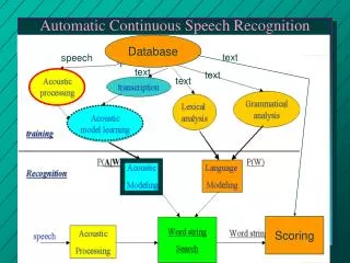
15. System Overview Courtesy of Bin Ma (2015)

16. System limitations inadequate training data (in speaker-dependent systems: user fatigue) • memory limitations • computation (searching among many possible texts) • inadequate models (poor assumptions made to reduce computation and memory, at the cost of reduced accuracy) • hard to train model parameters

17. Speech production • Speech: not an arbitrary signal • source of input to ASR: human vocal tract • data compression should take account of the human source • precision of representation: not exceed ability to control speech

18. Free variation • Aspects of speech that speakers do not directly control are free variation • Can be treated as distortion (noise, other sounds, reverberation) • Puts limits on accuracy needed • Creates mismatch between trained models and any new input • Intra-speaker: people never say the same exact utterance twice • Inter-speaker: everyone is different (size, gender, dialect,…) • Environment: SNR, microphone placement, … • Compare to vision PR: changes in lighting, shadows, obscuring objects, viewing angle, focus • Vocal-tract length normalization (VTLN); noise suppression

20. Speaker controls: amplitude, pitch, formants, voicing, speaking rate • Mapping from word (and phoneme) concepts in the brain to the acoustic output is complex • Trying to decipher speech is more complex than identifying objects in a visual scene • Vision: edges, texture, coloring, orientation, motion • Speech: indirect; not observing the vocal tract

21. Cues from perception • Auditory system sensitive to: dynamic positions of spectral peaks, durations (relative to speaking rate), fundamental frequency (F0) patterns • Important: where and when energy occurs • Less relevant: overall spectral slope, bandwidths, absence of energy • Formant tracking: algorithms err in transitions; not directly used in ASR for many years

22. Speech Signal Analysis • distribution of speech energy in frequency (spectral amplitude) • pitch period estimation • sampling rate typically: • 8 000/sec for telephone speech • 10 000 - 16 000/sec otherwise • usually 16 bits/sample • 8-bit mu-law logPCM (in the telephone network)

23. Short-time spectral analysis • Feature determination (e.g., formant frequencies, F0) requires error-prone methods • So, automatic methods (parameters) preferred: • FFT (fast Fourier transform) • LPC (linear predictive coding) • MFCC (mel-frequency cepstral coefficients) • RASTA-PLP • Log spectral (filter-bank) energies

26. Pitch (F0) estimation • Often, errors in weak speech and in transitions between voiced and unvoiced speech (e.g., doubling or halving F0) • peak-pick the time signal (look for energy increase at each closure of vocal cords) • usually first filter out energy above 1000 Hz (retain strong harmonics in F1 region) • often use autocorrelation to eliminate phase effects • often not done in ASR, due to the difficulty of exploiting F0 in its complex role of signaling different aspects of speech communication

27. Parameterization • Objective: model speech spectral envelope with few (8-16) coefficients • 1) Linear predictive coding (LPC) analysis: standard spectral method for low-rate speech coding • 2) Cepstral processing: common in ASR; also can exploit some auditory effects • 3) Vector Quantization (VQ): reduces transmission rate (but also ASR accuracy)

29. Cepstral processing • Cepstrum: inverse FFT of the log-amplitude FFT of the speech • small set of parameters (often 10-13) as LPC, but allows warping of frequency to match hearing • inverse DFT orthogonalizes • gross spectral detail in low-order values, finer detail in higher coefficients • C0: total speech energy (often discarded)

30. Cepstral coefficients • C1: balance of energy (low vs. high frequency) • C2,...C13 encode increasingly fine details about the spectrum (e.g., resolution to 100 Hz) • Mel cepstral coefficients (MFCCs) • model low frequencies linearly; above 1000 Hz logarithmically

31. Feature Transforms • Linear discriminant analysis (LDA) • As in analysis of variance (ANOVA), regression analysis and principal component analysis (PCA), LDA finds a linear combination of features to separate pattern classes • Maximum likelihood linear transforms • Speaker Adaptive Transforms • Map sets of features (e.g., MFCC, Spectral energies) to a smaller, more efficient set

32. Major issues in ASR • Segmenting speech spoken without pauses (continuous speech): • speech unit boundaries are not easily found automatically (vs.,e.g., Text-To-Speech) • Variability in speech: different speakers, contexts, styles, channels • Factors: real-time; telephone; hesitations; restarts; filled pauses; other sounds (noise, etc)

33. Comparing ASR tasks • speaker dependence • size of vocabulary • small (< 100 words) • medium (100-1000 words) • large (1-20 K words) • very large (> 20 K words) • complexity of vocabulary words • alphabet (difficult) • digits (easy)

34. Comparing ASR - 2 • allowed sequences of words - perplexity: mean # of words to consider - language models • style of speech: isolated words or continuous speech; how many words/utterance? • recording environment - quiet (> 30 dB SNR) - noisy (< 15 dB) - noise-cancelling microphone - telephone • real-time? feedback (rejection)? • type of error criterion • costs of errors

35. Possible ASR features • formants (e.g., F1 and F2) partition the vowels in the vowel triangle well (using F3 further minimizes overlap) • pitch (F0) • features are less commonly used in most ASR, owing to ASR to their complexity and difficulty of reliable estimation • Automatically determined bottleneck features in DNN • MFCC

36. ASR Thresholds • Thresholds: optional; to raise a ASR accuracy; cost = a delay • speaker allowed to repeat an utterance IF the best candidate has provided a poor match. • feasible for interactive ASR: immediate feedback or action. • balance ASR error rate and the “false rejection” rate (rejecting an otherwise correct response)

37. Temporal variability • Linear time alignment: simple mapping of long and short templates by linear compression or interpolation • Dynamic Time Warping: • - more costly method • - to accommodate natural timing variations in ordinary speech • - still used in some systems • Network methods: most widespread for the last 30 years

38. Dynamic Time Warping • Very popular in the 1970s • Compares exemplar patterns, with timing flexibility to handle speaking rate variations • No assumption of similarity across patterns for the same utterance • Thus, no way to generalize • Very poor to formulate efficient models

39. Hidden Markov Model (HMM) approach • Maximizing total ASR likelihood: “optimal” in that all input information is considered before global recognition decision made • Word-based HMMs: small-vocabulary applications • Phone-based HMMs: needed for large-vocabulary applications, due to difficulty of training, cost of computation and memory

41. HMM stochastic model • Bayes rule maximizes over possible {T}: • max P(T|S) = max[P(T)P(S|T)]/P(S) • Weight the decision by the a priori likelihood of text T being spoken (the Language Model) • Acoustic models P(S|T) for different speech units (words, phonemes, allophones)

42. Combining probabilities • For T frames, a = transitions, O = observations, i = states, b = state pdf’s:

43. for observation probabilities, usually Gaussian pdf's, • due to the simplicity of model, using only a mean and a variance • (in M dimensions, need a mean for each parameter, and • a MxM covariance matrix, noting the correlations between parameters)

44. Improving HMMs • major difficulty: first-order frame-independence assumption • use of delta coefficients over several frames (e.g., 50 ms) helps to include timing information, but is inefficient • stochastic trajectory models and trended HMMs are examples of ways to improve timing modeling • higher-order Markov models are too computationally complex • incorporate more information about speech production and perception into the HMM architecture?

45. Neural Networks

47. Long Short-Term Memory (LSTM) Memory Block Structure

50. Back-propagation in Time