Applied Economics for business management

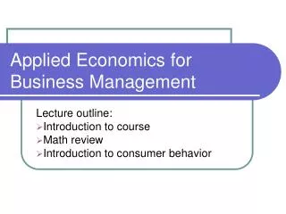
1. Applied Economics for business management Lecture #5

2. Lecture Outline Review Some topics in empirical estimation Start Supply

3. Empirical Estimation In the previous lecture, we briefly discussed heteroskedasticity, autocorrelation and multicollinearity as frequently encountered problems in empirical estimation. Perhaps more fundamental to these problems is specification error.

4. Specification Error Specification error in the broadest sense is any error in the model’s specification. In practice, specification error generally results from: (i) omission of relevant explanatory variables (ii) inclusion of irrelevant variables If a relevant variable is omitted from the estimating equation and is correlated with the other explanatory variables then the estimates of the misspecified equation are biased.

5. Example Consider the following example (Tomek and Robinson) concerning the estimation of the pork price equation:

6. See estimation results in table below:

7. Example Note the following: - as relevant variables are added the Durbin-Watson statistic (d) increases - the sign on income switches from negative to positive

8. Why are the coefficients on beef, chicken and turkey quantities negative? Because an increase in beef consumption implies a shift away from pork so the coefficient for a substitute is negative. Instead of deriving elasticities with quantity dependent demand equations, we can derive flexibilities with price dependent demand equations.

9. Flexibility Own price flexibility: Cross price flexibility: Inclusion of irrelevant variables does not produce bias but may increase the collinearity among explanatory variables.

10. Deflating In model specification, you as researchers will be faced with the question of whether or not to deflate and by what variable(s). In price analysis, deflating often involves dividing prices and/or income by some price index to derive real prices and income.

11. Deflating Why do we deflate? According to demand theory, demand equations should be homogeneous of degree zero by the homogeneity condition. This results in the absence of “money illusion”. So if all prices and income increase by 10%, the demand for commodities should not change.

12. Deflating An alternative to deflating is to include the product’s price and price deflator (index) as separate variables. Deflating a price series may not be necessary if the objective of the analysis is forecasting nominal commodity prices. For price forecasting, the researcher or analyst is forecasting the nominal price of the commodity. Leaving prices and income in nominal form (not deflated) and including the deflators in the estimating equation may produce possible multicollinearity problems.

13. Deflating Which deflator should one use? A common practice in demand analysis for a single food item is to divide the nominal price by the CPI (Consumer Price Index) for all items. For wholesale demand functions the common deflator has been the WPI (Wholesale Price Index) and for the farm level the deflator often used is the PPI (Producer Price Index).

14. Deflating A common practice in estimating aggregate consumption functions or systems of equations is to use the implicit price deflator based on the GNP (Gross National Product). The GNP deflator for a particular year contains all of the goods and services produced in the economy for that year. In contrast, the CPI measures the cost of a fixed bundle of goods whose composition does not vary over time except for periodic revision.

15. Dynamic Adjustment Models Much of the theory behind dynamic adjustment models come from: H.S. Houthakker and L.D. Taylor. 1970. Consumer Demand in the United States, 2nd edition, Harvard University Press. The classical theory of consumer demand assumes that the individual consumer tries to maximize utility or satisfaction subject to a budget constraint determined by commodity prices and consumer income. The limitation of this analysis has been the emphasis on a static approach.

16. Dynamic Adjustment Models Houthakker and Taylor suggest that consumers do not adjust instantaneously to price and income changes due to rigidities in consumer behavior and institutional restrictions. As a basis for dynamic analysis, Houthakker and Taylor (H-T) develop a model of consumer response influenced by past behavior, primarily habit formation and stock adjustment.

17. H-T Model The H-T model can be specified as:

18. H-T Model The H-T model can be specified as: The coefficient for lagged consumption provides a measure of the effects of habit formation and inventory adjustment. If the coefficient = 0 then this implies the absence of a dynamic adjustment effect.

19. H-T Model Two models are used in the H-T study: Because people do not adjust to price and income changes instantaneously, the partial adjustment toward can be represented as:

20. H-T Model λ is the adjustment coefficient or the per period proportion of adjustment toward the desired level.

21. H-T Model Substitute (2) into (4):

22. H-T Model This is the partial adjustment model that is estimated. Short-run price elasticity of demand evaluated at

23. H-T Model Long-run price elasticity of demand

24. H-T Model

25. H-T Model From equation (4): As λ gets closer to 0  adjustment is slower  longer adjustment period Using equation (4):  current period adjusts instantaneously to desired level and If λ approaches 1 then adjustment is faster  shortens the adjustment period

26. Production Economic Theory To derive the supply function for a given commodity, we have to begin with production by the firms in that industry. The theory of the firm for this course is the same as you would find in introductory and intermediate microeconomics courses.

27. Production Economic Theory Initially, we will assume that production occurs at a given point in time and space. We will also assume that there are no risks or uncertainties associated with production. Later in the course we will relax these assumption and cover topics such as production over time and production with risk and uncertainty.

28. Production Economic Theory We define the firm as an economic unit in which one or more products are produced. It is assumed that both product and factor markets are competitive, i.e., no firm or individual or group of firms or individuals have the ability to set product or factor prices. So the firm or entrepreneur is a price-taker.

29. Production Economic Theory What is production? Production can be described as the process by which resources are transformed into products or services. We usually refer to these resources as inputs or factors of production.

30. Production Economic Theory There are 2 general categories of inputs or factors of production: (i) fixed inputs (ii) variable inputs Fixed input are those inputs in the production process that cannot be increased or decreased in order to change the level of output for a given time period.

31. Production Economic Theory The most commonly used example of a fixed input is land. Generally, the amount of land is held constant during the production period. In the case of crops, the production period is the harvest season. Variable inputs are those inputs that can be varied in order to change the level of output for a given time period. There are numerous example of variable inputs: fertilizers, labor, pesticides, fuels, water applied, etc.

32. Production Economic Theory The distinction between fixed factors and variable factors of production depends on the time period of analysis. For instance, the amount of land in cultivation is fixed over a single harvest season but overtime, say in the next 5 years, the farmer may want to buy more land or sell some of his/her land. So a fixed input can become variable over time. The term production function or production process describes a physical relation between a firm’s inputs and its output of goods and services per unit time.

33. Production Economic Theory For this course, we will cover four production relationships: • factor-product case -- simplest case of one variable factor of production, some fixed inputs, and one product. (iv) factor-factor case -- two variable inputs, some fixed factors and one product. (v) product-product case -- one variable inputs, some fixed factors and 2 products. (vi) general case -- m variable inputs, some fixed factors and n products.

34. Production Economic Theory • Factor-product case: • Some assumptions: • Production function is continuous with continuous first • and second derivatives. • (ii) Inputs and outputs are non-negative. • (iii)Production function represents the current state of the • art.

35. Production Economic Theory • Production function represents the • current state of the art. • What does the third assumption imply?

36. Production Economic Theory With the state of the art technology, the producer can produce output However, point c represents an inefficient use of resource

37. Production Economic Theory With the given state of the art technology, the producer cannot produce output

38. Production Economic Theory • Fixed inputs do not alter the quantity of output • produced during the production period under consideration. • (v) Inputs and outputs are expressed per unit of time. For • example, in specifying alfalfa hay production as 4 tons • per acre it is important to know whether this is 4 • tons/acre/year or 4 tons/acre/decade.

39. Production Economic Theory The production function can be written as: where / separates the variable input from the fixed inputs. For this production function, we have one variable input and fixed inputs.

40. Production Economic Theory We generally define certain physical relationships in production as follows: TPP = total physical product or output e.g., lbs of beef produced, tons of alfalfa hay produced, etc. APP = average physical product MPP = marginal physical product

41. Production Economic Theory Problem: Production managers for Cosmic Paper Corporation estimate that their production process is currently characterized by the following production function:

42. Production Economic Theory Problem: Production managers for Cosmic Paper Corporation estimate that their production process is currently characterized by the following production function: a) Write the corresponding MPP and APP functions for input b) What is the MPPx when • At what value of maximized? • Be sure to verify sufficient conditions.

43. Production Economic Theory a) Write the corresponding MPP and APP functions for input

44. Production Economic Theory b) What is the MPPx when

45. Production Economic Theory • At what value of maximized? • Be sure to verify sufficient conditions. c. Maximize q 

46. Production Economic Theory Use 2nd derivative test: