Network calculus ( system theory )

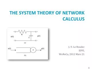
Network calculus( system theory ) Jean-Yves Le Boudec ICA, EPFL CH-1015 Lausanne jean-yves.leboudec@epfl.ch http://icawww.epfl.ch

Contents • 1. background material • 2. the greedy shaper viewed as a min-plus system • 3. min-plus operators and a theorem • 4. the packetized shaper • 5. other examples

Part 1: Background MaterialArrival and Service Curves • Internet integrated and differentiated services use the concepts of arrival curve and service curves

Arrival Curves • Arrival curve  R(t) -R(s) (t-s) Examples: • leaky bucket (u) = ru+b • standard arrival curve in the Internet(u) = min (pu+M, ru+b) bits slope r b slope m time M

Arrival Curves can be assumed sub-additive • Theorem: can be replaced by a sub-additive function • sub-additive: (s+t) (s) + (t) • concave => subadditive

Service Curve • System S offers a service curve  to a flow iff for all t there exists some s such that R R*(t) R(s) R* s t

buffer s t The constant rate server has service curve b(t)=ct Proof: take s = beginning of busy period: R*(t) – R*(s) = c (t-s) R*(t) – R(s) = c (t-s)

R R* T (t)  T 0 T t seconds Function T The guaranteed-delay node has service curve dT

The standard model for an Internet router • rate-latency service curve bits R T seconds

fresh traffic shaped traffic s-smooth s R R* Part 2: The Greedy Shaper viewed as a Min-Plus System • shaper: forces output to be constrained by  • greedy shaper storesdata in a buffer only if needed • examples: • constant bit rate link (s(t)=ct) • ATM shaper; fluid leaky bucket controller • Pb: find input/output relation

fresh traffic shaped traffic s-smooth s R x A Min-Plus Model for Shapers • Shaper Equations: (1) x  x (2)x  R

(1) x  x  (2)x  R Solving the Min-Plus Model • Theorem: There is a maximum solution; it is equal to R  • Proof: (1) find a solution: fixed point x0 = R ; xi = xi-1 and x* = inf {x0, x1, ..., xi, ...} here:  =  and thus xi = R =x* (2) if x is a solution, then x  R thus x   R 

fresh traffic shaped traffic s-smooth s R R* I/O of Greedy Shaper • for any shaper, output R  • R is wide-sense increasing, thusR  also • thus: the greedy shaper output is R*= R 

fresh traffic constrained by a re-shaped traffic s R R* A consequence: Greedy Shaper Keeps Arrival Constraints • The output of the shaper is still constrained by  • ProofR* = R  (R R R* 

Part 3: Min-Plus Operators and a theorem • G = set offunctions R -> R+ that are wide-sense increasing • works also if time is discrete: N -> R+ • we consider operators  : G -> G •  is isotone if x(t)y(t)=> (x)(t) (y)(t) •  is upper-semi continuous iff infi((xi )) = (infi(xi)) for  sequences xi

Min-Plus Linear Operators •  is min-plus linear if • for any constant K, (x + K) = (x) + K (x  y) = (x)  (y) •  is upper-semi continuous. • Representation Theorem:  is min-plus linear <=>there is some H: R x R -> R+ such that (x)(t)=infs[H(t,s)+x(s)] • min-plus linear => isotone

Other Properties of Operators •  is time invariant if for some T y(t) = (x)(t) and x’(t) = x(t+T) => (x’)(t) = y(t+T) •  is causal if (x)(t) depends only onx(s), 0  s  t

Two linear operators • Convolution by a fixed function: Cs:x -> x  s • Cs is linear, time invariant, not causal • Cso Cs’ = Css’ • Idempotent operator hM x-> hM (x)with hM(t) = infst { M(t)- M(s) + x(s) } • is idempotent: hMo hM = hM • linear, causal, not time invariant

The Packetizer • Define function PL byPL(x) = L(n)  L(n)  x < L(n+1) [Chang 99] • call PL the operator: PL(R)(t) = PL(R(t)) accumulates bits until entire packets can be delivered • PL is idempotent, not linear, but is isotone and upper-semi continuous

A Min-Plus Theorem • Implicitely contained in Baccelli et al, “Synchronization and Linearity”, Baccelli et al. • Theorem: Assume that  is isotone and upper-semi-continuous. Theproblemx(t)b(t) (x)(t) has one maximum solution in G, given by x*(t)= (b)(t) • (Definition of closure)  (x) = inf {x, (x), (x), (x),...} • in other words: x0 = b ; xi =  (xi-1) and x* = inf {x0, x1, ..., xi, ...}

fresh traffic shaped traffic s-smooth s R R* Part 4: packetized shaper • same as previous, but releases only entire packets • example : leaky bucket controller • Pb: find input/output relation of packetized greedy shaper

fresh traffic shaped traffic s-smooth s R R* Model for packetized shapers • Define L(i) = l1 + l2 + … + li • The output satisfies: (1) R*  R* (2)R*  R (3) R* is L-packetized

Modelling packetized greedy shapers • system equation : R*PL (R*)C(R*)  R • maximum solution: R* = PL C(R) • th 4.3.3: closure ((PId)o(QId))= closure(PQ)thus closure(PL C)=closure(PL oC) • after some algebra:R* = inf {R(1) , R(2), R(3), …} with R(i)= PL oC o … o PL oC (R)i.e. R(0)=R, R(i) = PL(R(i-1))

5 4 3 1 2 0 R(1) R(2) R(3) R* = R(4) Numerical Example for R* = PL C(R) • (t) = 25  t/T  for t >0, else 0 •  - smooth<=> at most 25 data unit per time unit • R(t)= a burst of 10 packets of size 10 at time 0 • R(i) = PL(R(i-1))

Special Case • Theorem (LeBoudec, Sigmetrics 2001)If s = s0 + l with l  lmax then PL oC o … o PL oCs = PL oC oPLand thus R* = PL(R) • Applications: if  is concave and (0+)  lmax then the packetized shaper can be realized as the concatenation : shaper + packetizer • leaky bucket controllers based on bucket replenishment are functionally equivalent to leaky bucket based on virtual finish times

fresh traffic m(t) R R* Part 5: Other ExamplesEx3: Variable Capacity Node • node has a time varying capacity µ(t)Define M(t) =0tm(s) ds. • the output satisfies R*  R R*(t) -R*(s)  M(t) -M(s) for all s  tand is “as large as possible”

fresh traffic m(t) R R* Variable Capacity Node • R*  RR*(t) -R*(s)  M(t) -M(s) for all s  t • R* R hM(R*) • thus there is a maximum solution in G, and R*= hM(R) • now hR is idempotent thus hM = hM • finally: R*(t) = infst { M(t)- M(s) + R(s) }

Loss L(t) fresh traffic R(t) b R’(t) buffer X R*(t) Ex 4: Loss System • node with service curve b(t) and buffer X • when buffer is full incoming data is discarded • modelled by a virtual controller (not buffered) • fluid model or fixed sized packets • Pb: find loss ratio

Loss L(t) fresh traffic R(t) b R’(t) buffer X R*(t) Model for Loss System • R’(t) satisfies R’  (X + P(R’))h R(R’) d0 where P is the transformation R’ -> R* • assume P isotone and usc (« physical assumptions »); thus R’ = (X + P ) h R(d0) • we don’t know P but P Cb • theorem:PP’ => PP’ • thus R’  (X + Cb) h R(d0)

Loss L(t) fresh traffic R(t) b R’(t) buffer X R*(t) Representation of Loss • we have shown: R’  (X + Cb) h R(d0) • compute the closure, obtain R’, thus the loss process L=R-R’

Bound on Loss Ratio • Theorem: if R is a-smooth, then L(t)/R(t) 1 - r with r = min(1, inf t  0 [b(t) +X] /a(t)) • best bound with these assumptions • proof: • define x(t) = r R(t) • x satisfies the system equation:x  (X + xb)  h R(x) (X + P(x))h R(x) • R’ is the maximum solution=> x(t)  R’(t) for all t

Video server Video display Network Smoother R(t) R’(t) R*(t) R(t-D)  ß(t) B s Ex 5: Optimal smoothing • Network offers a service curve b to flow R’(t), • Smoother delivers a flow R’(t) conforming to an arrival curve s. • Video stream is stored in the client buffer B read after a playback delay D. • Pb: which smoothing strategy minimizes D and B ?

Video server Video display Network Smoother R(t) R’(t) R*(t) R(t-D)  ß(t) B s System Equations • (1) R’ is s-smooth • (2) (R’(t)  R(t-D) • R’(t) = 0 for t  0 • Define min-plus deconvolution (a Ø b)(t) =sups 0[a(s+t)-b(s)] • x  y   <=> x Ø  y

Max-Plus operators • replace  by , min-plus becomes max-plus • Deconvolution with a fixed function x -> x Ø ais max-plus linear

Video server Video display Network Smoother R(t) R’(t) R*(t) R(t-D)  ß(t) s A max-plus model for Example 5 • R’ satisfies: (1) R’  R’ Ø s (2)R’  (R Ø  )(t-D) • a max-plus system, , withminimum solution x* = inf {x0, x1, ..., xi, ...} x0 (t) = (R Ø  )(t-D) xi = xi-1Ø s • thus R’ = (R Ø  )Ø s (t-D) = R Ø ( s) (t-D)

* 106 5 4 3 2 1 R(s  b) -50 0 50 100 150 200 250 300 350 400 450 minimum value of D Frame # Example s  b(t) R(t)

Minimum Playback Delay • D must satisfy :R Ø ( s) (-D)  0 • this is equivalent to D  h(R,  s)

* 106 5 4 3 2 1 D=h(R,s  b) s  b(t) R(t) -50 0 50 100 150 200 250 300 350 400 450 Frame # Back to our example

R(t) 70 10000 60 50 40 8000 30 20 10 6000 100 200 300 400 (s  b)(t) (s  b)(t) 4000 2000 100 200 300 400 10000 70 8000 60 6000 50 40 4000 30 2000 20 10 100 200 300 400 100 200 300 400 D = 435 ms D = 102 ms

bits bits bits bits R(t) R(t) R() R() R( ) R( ) S(t) R  (s  b ) S s  b R(t) T T T T (3) Shape with s  b s  b Deconvolution is the time inverse of convolution (4) Invert time again (2) S(t) in inverted time (1) R(t) in real time

* 106 5 4 3 2 1 R (s  b) -50 0 50 100 150 200 250 300 350 400 450 Frame # Back to our example • Infocom 2001: Joint Smoothing and Source Rate Selection (Verscheure, Frossard, Le Boudec) R(t)

Conclusion • Network Calculus is a set of tools and theories for the deterministic analysis of communication networks • Application of min-plus algebra • Does not supersede stochastic queueing analysis, but gives new tools for analysis of sample paths • Book and slides available online at Le Boudec’s or Thiran’s home page

Network calculus ( system theory )