Download
1 / 48
500 likes | 810 Views
Introduction to Graphs. INTRODUCTION. Line graphs illustrate the relationships between two variables, showing graphically what happens to one variable when the other changes. Representation of equations by means of graphs They give a visual picture of the behaviour of the two variables

E N D
INTRODUCTION • Line graphs illustrate the relationships between two variables, showing graphically what happens to one variable when the other changes. • Representation of equations by means of graphs • They give a visual picture of the behaviour of the two variables • Graphical approaches to problem solving are often easier to carry out than mathematical ones • They are less accurate, since the answers must be read from the graph and hence cannot be more accurate than the thickness of the pencil
BASIC PRINCIPLES OF GRAPHS • A graph is a diagram illustrating one or more mathematical relationships between two variables. • The y-axis is the vertical axis and usually displays the dependent variable – i.e. the variable which changes according to changes in the other variable • he x-axis is the horizontal axis and usually displays the independent variable – i.e. the variable which causes change in the other variable. • Scale used must be clear to the reader. • The scale need not be the same on both axes. • Each axis should be titled to show clearly both what it represents and the units of measurement.
The area within the axes (known as the plot area) is divided into a grid by reference to the scale on the axes. • Particular points within the graph are identified by a pair of numbers called co-ordinates which fix a point by reference to the scales along the axes. The first co-ordinate number always refers to a value on the scale along the x-axis and the second to the scale on the y- axis • The point at which the two axes meet is called the origin. This has the co-ordinate reference (0,0). • Finally, note that the x and y-axes may extend to include negative numbers
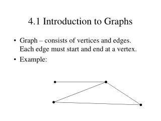
Drawing a Graph • Determine the range of values which will need to be shown on each of the axes. • Draw the axes and mark off the scales along them. • The aim is usually to draw as large a graph as possible since this will make it easier to plot the co-ordinates accurately, and also make it easier to read • The scales must be consistent along each axis, but do not need to be the same on both • Give each axis a title, number the main divisions along each scale and give the whole graph a title.
Representation • The values in the table can be expressed as a pair of co-ordinates which may be plotted on a graph. The first figure is the value of x along the scale of the x (horizontal) axis, and the second figure is the value of y along the scale of the y (vertical) axis • Ordered Pairs : Another way of describing the varying values of x and y is by means of a set of ordered pairs. This is a very useful and helpful way of noting the points we required in the graphical representation of a function
Characteristics of Straight-Line Graphs • Lines parallel to an axis • Lines through the origin • Parallel lines • Direction of slope • Intercepts
Gradient of a Straight Line • We can easily calculate the gradient of a straight line joining two points from the co-ordinates of those points.
USING GRAPHS IN BUSINESS PROBLEMS • Business Costs
Economic Ordering Quantities • One of the central issues in purchasing materials to be used as part of the production process is how much to order and when. Many producers and most retailers must purchase the materials they need for their business in larger quantities than those needed immediately. • However, there are costs in the ordering of materials – for example, each order and delivery might incur large administrative and handling costs, including transportation costs, so buying in stock on a daily basis might not be appropriate. On the other hand, there are also costs involved in holding a stock of unused materials – very large stocks can incur large warehousing costs. Set against this, buying in larger quantities has the effect of spreading the fixed costs of purchase over many items, and can also mean getting cheaper prices for buying in bulk. The purchaser must determine the optimum point. • By "economic order quantity" we mean the quantity of materials that should be ordered in order to minimize the total cost.
Plotting Time Series Data • Businesses and governments statistically analyze information and data collected at regular intervals over extensive periods of time, to plan future strategies and policies. For example, sales values or unemployment levels recorded at yearly, quarterly or monthly intervals could be examined in an attempt to predict their future behaviour. Such sets of values observed at regular intervals over a period of time are called time series • The analysis of this data is a complex problem as many variable factors may influence the changes which take place. The first step in analyzing the data is to plot the observations on a scattergram, with time evenly spaced across the x-axis and measures of the dependent variable forming the y-axis. This can give us a good visual guide of the trend in the time series data.