
Spatial Analysis Techniques for Environmental Studies
E N D
Presentation Transcript
Chapter 10 Problems Even problems are at end of text. 19. What is a kernel in a moving window operation? Does the kernel size or shape change for different portions of the data set? Why or why not? Lecture 12
23. Calculate the cost of travel between A and B, and A and C. A to B A to C Lecture 12
Chapter 11 Problems Answers to even numbered problems are in the back of the text. 3. Define slope and aspect and give the mathematical formulas used to derive them from elevation data. Slope is the change in elevation compared to a change in the horizontal position. Lecture 12
Aspect is the direction of the slope. Lecture 12
Lab 5 – Spatial Analysis • Will be up on the website later today. • You will be creating your own Report Sheet. • 10 screen shots plus a layout. Lecture 12
Uncheck all layers except for the one you are screen printing. • Crop the image. • Set the size to 3” • Total pages I am willing to print per this lab is 4. Lecture 12
Spatial Estimation Chapter 12 – Part 1 Lecture 12
Introduction • Spatial prediction methods are used to estimate values at un-sampled locations. • Not all locations can be sampled: • Time • Money • An infinite number of samples or a large finite number of samples. • Locations are difficult or impossible to get to. • Missing or suspect data. Lecture 12
Spatial Interpolation • The prediction of variables at unmeasured locations based on the sampling of the same variables at known location. • Soil temperature • Elevation • Ocean productivity Lecture 12
Spatial Prediction • The estimation of variables at un-sampled locations based, at least in part, on other variables, and often on a total set of measurements. • Elevation as a proxy for temperature. • Soil nitrogen content as a proxy for crop yield. Lecture 12
Spatial Prediction (cont’d) • Usually translates to same or higher dimension: • Point data to point or line data • In the opposite direction we have the MAU problem. 250 deer 1000 deer Lecture 12
Core Area • A high use, density, intensity or probability of the occurence of a variable or an event. • A core area is defined from a set of samples and are used to predict the frequency or likelihood of the occurence of an object or event. • Location of traffic accidents • High crime areas Lecture 12
Sampling • Sampling • A shortcut method for investigating a whole population • Data is gathered on a small part of the whole parent population or sampling frame, and used to inform what the whole picture is like • We control the number of samples and the pattern • Common sampling patterns in spatial analysis: • Systematic • Random • Cluster • Adaptive Lecture 12
Systematic sampling pattern Easy Samples spaced uniformly at fixed X, Y intervals Parallel lines Advantages Easy to understand Disadvantages All receive same attention Difficult to stay on lines May be biases Lecture 12
Random Sampling Select point based on random number process Plot on map Visit sample Advantages Less biased (unlikely to match pattern in landscape) Disadvantages Does nothing to distribute samples in areas of high Difficult to explain, location of points may be a problem Lecture 12
Cluster Sampling Cluster centers are established (random or systematic) Samples arranged around each center Plot on map Visit sample (e.g. US Forest Service, Forest Inventory Analysis (FIA) Clusters located at random then systematic pattern of samples at that location) Advantages Reduced travel time Lecture 12
Adaptive sampling More sampling where there is more variability. Need prior knowledge of variability, e.g. two stage sampling Advantages More efficient, homogeneous areas have few samples, better representation of variable areas. Disadvantages Need prior information on variability through space Lecture 12
INTERPOLATION Many methods - All combine information about the sample coordinates with the magnitude of the measurement variable to estimate the variable of interest at the unmeasured location Methods differ in weighting and number of observations used Different methods produce different results No single method has been shown to be more accurate in every application Accuracy is judged by withheld sample points Lecture 12
INTERPOLATION Outputs typically: Raster surface • Values are measured at a set of sample points • Raster layer boundaries and cell dimensions established • Interpolation method estimate the value for the center of each unmeasured grid cell Contour Lines Iterative process • From the sample points estimate points of a value Connect these points to form a line • Estimate the next value, creating another line with the restriction that lines of different values do not cross. Lecture 12
Example Base Lecture 12 Elevation contours Sampled locations and values
INTERPOLATION 1st Method - Thiessen Polygon Assigns interpolated value equal to the value found at the nearest sample location Conceptually simplest method Only one point used (nearest) Often called nearest sample or nearest neighbor Lecture 12
INTERPOLATION Thiessen Polygon Advantage: Ease of application Accuracy depends largely on sampling density Boundaries often odd shaped as transitions between polygons are often abrupt Continuous variables often not well represented Lecture 12
Thiessen Polygon Draw lines connecting the points to their nearest neighbors. Find the bisectors of each line. Connect the bisectors of the lines and assign the resulting polygon the value of the center point Source: http://www.geog.ubc.ca/courses/klink/g472/class97/eichel/theis.html Lecture 12
3 1 2 Start: 1) 5 4 2) 3) Thiessen Polygon • Draw lines connecting the points to their nearest neighbors. • Find the bisectors of each line. • Connect the bisectors of the lines and assign the resulting polygon the value of the center point Lecture 12
Sampled locations and values Thiessen polygons Lecture 12
INTERPOLATION Fixed-Radius – Local Averaging More complex than nearest sample Cell values estimated based on the average of nearby samples Samples used depend on search radius (any sample found inside the circle is used in average, outside ignored) • Specify output raster grid • Fixed-radius circle is centered over a raster cell Circle radius typically equals several raster cell widths (causes neighboring cell values to be similar) Several sample points used Some circles many contain no points Search radius important; too large may smooth the data too much Lecture 12
INTERPOLATION Fixed-Radius – Local Averaging Lecture 12
INTERPOLATION Fixed-Radius – Local Averaging Lecture 12
INTERPOLATION Fixed-Radius – Local Averaging Lecture 12
INTERPOLATION Inverse Distance Weighted (IDW) Estimates the values at unknown points using the distance and values to nearby know points (IDW reduces the contribution of a known point to the interpolated value) Weight of each sample point is an inverse proportion to the distance. The further away the point, the less the weight in helping define the unsampled location Lecture 12
INTERPOLATION Inverse Distance Weighted (IDW) Zi is value of known point Dij is distance to known point Zj is the unknown point n is a user selected exponent Lecture 12
INTERPOLATION Inverse Distance Weighted (IDW) Lecture 12
INTERPOLATION Inverse Distance Weighted (IDW) Factors affecting interpolated surface: • Size of exponent, n affects the shape of the surface larger n means the closer points are more influential • A larger number of sample points results in a smoother surface Lecture 12
INTERPOLATION Inverse Distance Weighted (IDW) Lecture 12
INTERPOLATION Inverse Distance Weighted (IDW) Lecture 12
INTERPOLATION Splines Name derived from the drafting tool, a flexible ruler, that helps create smooth curves through several points Spline functions are use to interpolate along a smooth curve. Force a smooth line to pass through a desired set of points Constructed from a set of joined polynomial functions Lecture 12
Spline • Surface created with Spline interpolation • Passes through each sample point • May exceed the value range of the sample point set Lecture 12
INTERPOLATION : Splines Lecture 12
Measuring Interpolation Accuracy • Hold back 10% of the sample points. • Create your interpolated surface. • Add the withheld points, how well did the surface predict the values of the withheld points. Lecture 12
Interpolation vs. Prediction • Spatial prediction is more general than spatial interpolation. • Both are used to estimate values of a variable at unknown locations. • Interpolation use only the measured target variable and sample coordinates to estimate the variable at unknown locations. • Prediction methods address the presence of spatial autocorrelation. Lecture 12
Tobler’s Law Tobler's First Law of Geography. A formulation of the concept of spatial autocorrelation by the geographer Waldo Tobler (1930-), which states: "Everything is related to everything else, but near things are more related than distant things." Lecture 12
Spatial Prediction • Based on mathematical models often built by a statistical process. • Distinction between interpolation and prediction may be viewed as artificial, but it can be more general than interpolation. • In addition to autocorrelation, variables may show cross-correlation, the tendency for two variables to change together. Lecture 12
Spatial autocorrelation: Higher autocorrelations, points near each other are alike. Lecture 12
Cross-correlation – two variables change in concert (positive or negative) Lecture 12
Moran’s I – A Measure of Spatial Correlation Lecture 12
Moran’s I (cont’d) • Moran’s I approaches a value of +1 in areas of positive spatial correlation: • Large values tend to be clumped together. • Small values tend to be clumped together. • Values approach 0 in areas of low spatial correlation. • A value of -1 are anti-correlated, a large value is next to a small value. Lecture 12
Spatial Prediction Trend Surface Fitting a statistical model, a trend surface, through the measured points. (typically polynomial) Where Z is the value at any point x Where ais are coefficients estimated in a regression model Lecture 12
Spatial Prediction Trend Surface Lecture 12