Understanding Production Externalities and Efficient Regulation
120 likes | 231 Views
Learn about production externalities and the impact on output, social welfare, and environmental costs. Explore policies like taxes, quotas, and subsidies to correct market failures efficiently. Exercises and examples illustrate the concepts.

Understanding Production Externalities and Efficient Regulation
E N D
Presentation Transcript
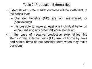
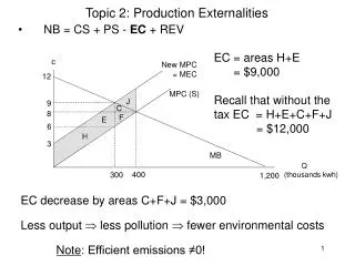
Topic 2: Production Externalities EC = areas H+E = $9,000 Recall that without the tax EC = H+E+C+F+J = $12,000 c New MPC = MEC 12 • NB = CS + PS - EC + REV MPC (S) J 9 C 8 F E 6 H 3 MB Q (thousands kwh) 400 300 1,200 EC decrease by areas C+F+J = $3,000 Less output less pollution fewer environmental costs Note: Efficient emissions ≠0!
Topic 2: Production Externalities REV = areas B+D+E = $9,000 Without the tax REV = 0 (obviously) c New MPC = MEC 12 • NB = CS + PS - EC + REV MPC (S) 9 B 8 D E 6 Tax-payers gain $9,000. 3 MB Q (thousands kwh) 400 300 1,200 Note that REV = t Q = MEC Q Recall that EC = MEC Q REV = EC (because MEC is constant in Q)
Topic 2: Production Externalities Combined gains in terms of EC and REV: c New MPC = MEC EC + REV = areas B+C+D+E+F+J = $3,000 + $9,000 = $12,000 12 MPC (S) J 9 B C 8 F D E 6 3 MB Q (thousands kwh) 400 300 1,200 Recall: combined losses to CS and PS were = B+C+D+E+F = $10,500. Gains exceed losses by $1,500 = J. Area J was DWL.
Topic 2: Production Externalities • Summary of effects of per unit tax on output: • If we set t = MEC: • The efficient Q is achieved. • Losses in terms of CS and PS • Gains in terms of REV and EC • Relevant question for policy: • What information does the environmental regulator need in order to be able to implement this policy? • If MEC is constant in Q, then we just need to know what that MEC is equal to. • No requirement to know MPC or MB (demand). Gains > Losses NB
Topic 2: Production Externalities • Exercise (more difficult): • Suppose we have the same MB and same MPC curves as in the previous example, but now suppose that MEC = (1/100)Q (that is, as Q , MEC ). • Questions: • What is the efficient level of output? Draw a diagram. • Calculate the DWL that results at the equilibrium if there is no policy to correct the market failure. • If the government wishes to correct the market failure by setting a constant per unit output tax, what will that tax need to be? • Calculate the CS, PS, EC, REV as result of this tax. • What new information does the regulator need in this case (relative to the case of constant MEC) in order to achieve efficiency?
Topic 2: Production Externalities • Quota on production • Now suppose we want to achieve efficiency, but through a quota on production rather than a per unit output tax. • If we limit output per power plant to 3,000 kwh, then aggregate Q cannot exceed 300,000 (the efficient Q). • Questions: • What is the new equilibrium P and Q? • Who gains and who loses as a result of the quota? • What information does the regulator need in order to achieve the efficient Q?
Topic 2: Production Externalities Effect of a quota on the market for electricity: If aggregate Q cannot exceed 300, then P to $0.09. Effect on CS identical to effect of t=$0.03. c MEC 12 MPC 9 8 3 MB Q (thousands kwh) 400 300 1,200 Effect on EC identical to effect of t=$0.03. What about PS? Exercise: Calculate the PS and show that PS + EC > CS by an amount equal to the initial DWL. Also, what information does the regulator need in this case?
Topic 2: Production Externalities • Per unit subsidy on output reduction. • Finally, suppose we want to achieve efficiency, but by paying producers to reduce their output. • Key point to understand: • A subsidy on Q increases the firm’s MPC in (more or less) the same way a tax does. • The subsidy increases the opportunity cost to the firm. • If the firm decides to produce an extra unit of Q, the firm must pay its MPC, but now must also forgo the subsidy.
Topic 2: Production Externalities • In our example, each firm chooses Q = 4,000 with no regulation. • Suppose the govt offers to pay each firm $0.03 for every unit it doesn’t produce, below the baseline output of Q = 4,000. • Example: if a firm chooses Q = 3,800, it receives the subsidy on 200 units (i.e., it receives a payment of $6.00), etc.
Topic 2: Production Externalities Effect on an individual firm of a subsidy on Q reduction: c MPC with sub on Q MSC Govt pays firm $0.03 per kwh not produced below 4000. MPC for all Q < 4,000. MPC 3 Q (thousands kwh) 4 If Q < 4,000, the cost to the firm of an extra Q = MPC + subsidy forgone = MPC + $0.03 = MSC
Topic 2: Production Externalities Effect on electricity market of a subsidy on Q reduction: New equilibrium is at Q = 300, with consumers paying P =$0.09 per unit. c MSC 12 9 MPC Effect on CS and EC will be the same as with the tax and quota. 3 MB Q (thousands kwh) 300 400 Exercise: By how much does PS? How much does REV? Identify the areas corresponding to PS & REV. Show that PS + EC > CS + REV by an amount equal to the initial DWL. What info does the regulator need in this case?