Download
1 / 61
610 likes | 749 Views
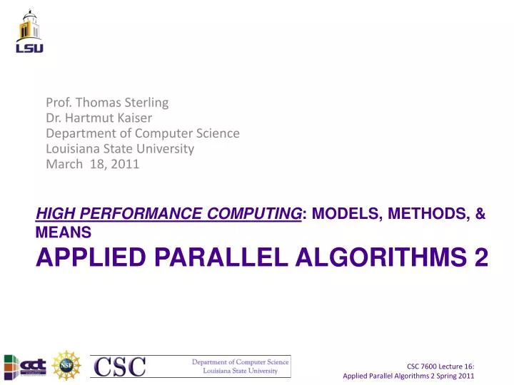
Prof. Thomas Sterling Dr. Hartmut Kaiser Department of Computer Science Louisiana State University March 18, 2011. HIGH PERFORMANCE COMPUTING : MODELS, METHODS, & MEANS APPLIED PARALLEL ALGORITHMS 2. Puzzle of the Day. if(a = 0) { … }

E N D
Prof. Thomas Sterling Dr. Hartmut Kaiser Department of Computer Science Louisiana State University March 18, 2011 HIGH PERFORMANCE COMPUTING: MODELS, METHODS, & MEANSAPPLIED PARALLEL ALGORITHMS 2
Puzzle of the Day if(a = 0) { … } /* a always equals 0, but block will never be executed */ if(0 < a < 5) { … } /* this "boolean" is always true! [think: (0 < a) < 5] */ if(a =! 0) { … } /* a always equal to 1, as this is compiled as (a = !0), an assignment, rather than (a != 0) or (a == !0) */ Some nice ways to get something different from what was intended:
Topics Array Decomposition Matrix Transpose Gauss-Jordan Elimination LU Decomposition Summary Materials for Test
Topics Array Decomposition Matrix Transpose Gauss-Jordan Elimination LU Decomposition Summary Materials for Test
Parallel Matrix Processing & Locality Maximize locality Spatial locality Variable likely to be used if neighbor data is used Exploits unit or uniform stride access patterns Exploits cache line length Adjacent blocks minimize message traffic Depends on volume to surface ratio Temporal locality Variable likely to be reused if already recently used Exploits cache loads and LRU (least recently used) replacement policy Exploits register allocation Granularity Maximizes length of local computation Reduces number of messages Maximizes length of individual messages
Array Decomposition Simple MPI Example Master-Worker Data Partitioning and Distribution Array decomposition Uniformly distributes parts of array among workers (and master) A kind of static load balancing Assumes equal work on equal data set sizes Demonstrates Data partitioning Data distribution Coarse grain parallel execution No communication between tasks Reduction operator Master-worker control model
Array Decomposition Layout Dimensions 1 dimension: linear (dot product) 2 dimensions: “2-D” or (matrix operations) 3 dimensions (higher order models) Impacts surface to volume ratio for inter process communications Distribution Block Minimizes messaging Maximizes message size Cyclic Improves load balancing Memory layout C vs. FORTRAN
Array Decomposition Accumulate sum from each part
Array Decomposition Demonstrate simple data decomposition : • Master initializes array and then distributes an equal portion of the array among the other tasks. • The other tasks receive their portion of the array, they perform an addition operation to each array element. • Each task maintains the sum for their portion of the array • The master task does likewise with its portion of the array. • As each of the non-master tasks finish, they send their updated portion of the array to the master. • An MPI collective communication call is used to collect the sums maintained by each task. • Finally, the master task displays selected parts of the final array and the global sum of all array elements. • Assumption : that the array can be equally divided among the group.
Flowchart for Array Decomposition “master” “workers” … Initialize MPI Environment Initialize MPI Environment Initialize MPI Environment Initialize MPI Environment Initialize Array Partition Array into workloads Send Workload to “workers” … Recv. work Recv. work Recv. work … Calculate Sum for array chunk Calculate Sum for array chunk Calculate Sum for array chunk Calculate Sum for array chunk … Send Sum Send Sum Send Sum Recv. results Reduction Operator to Sum up results Print results End
Array Decompositon (source code) #include "mpi.h" #include <stdio.h> #include <stdlib.h> #define ARRAYSIZE 16000000 #define MASTER 0 float data[ARRAYSIZE]; int main (int argc, char **argv) { int numtasks, taskid, rc, dest, offset, i, j, tag1, tag2, source, chunksize; float mysum, sum; float update(int myoffset, int chunk, int myid); MPI_Status status; MPI_Init(&argc, &argv); MPI_Comm_size(MPI_COMM_WORLD, &numtasks); if (numtasks % 4 != 0) { printf("Quitting. Number of MPI tasks must be divisible by 4.\n"); /**For equal distribution of workload**/ MPI_Abort(MPI_COMM_WORLD, rc); exit(0); } MPI_Comm_rank(MPI_COMM_WORLD,&taskid); printf ("MPI task %d has started...\n", taskid); chunksize = (ARRAYSIZE / numtasks); tag2 = 1; tag1 = 2; Workload to be processed by each processor Source : http://www.llnl.gov/computing/tutorials/mpi/samples/C/mpi_array.c
Array Decompositon (source code) if (taskid == MASTER){ sum = 0; for(i=0; i<ARRAYSIZE; i++) { data[i] = i * 1.0; sum = sum + data[i]; } printf("Initialized array sum = %e\n",sum); offset = chunksize; for (dest=1; dest<numtasks; dest++) { MPI_Send(&offset, 1, MPI_INT, dest, tag1, MPI_COMM_WORLD); MPI_Send(&data[offset], chunksize, MPI_FLOAT, dest, tag2, MPI_COMM_WORLD); printf("Sent %d elements to task %d offset= %d\n",chunksize,dest,offset); offset = offset + chunksize; } offset = 0; mysum = update(offset, chunksize, taskid); for (i=1; i<numtasks; i++) { source = i; MPI_Recv(&offset, 1, MPI_INT, source, tag1, MPI_COMM_WORLD, &status); MPI_Recv(&data[offset], chunksize, MPI_FLOAT, source, tag2, MPI_COMM_WORLD, &status); } Initialize array Array[0] -> Array[offset-1] is processed by master Send workloads to respective processors Master computes local Sum Master receives summation computed by workers Source : http://www.llnl.gov/computing/tutorials/mpi/samples/C/mpi_array.c
Array Decompositon (source code) MPI_Reduce(&mysum, &sum, 1, MPI_FLOAT, MPI_SUM, MASTER, MPI_COMM_WORLD); printf("Sample results: \n"); offset = 0; for (i=0; i<numtasks; i++) { for (j=0; j<5; j++) printf(" %e",data[offset+j]); printf("\n"); offset = offset + chunksize; } printf("*** Final sum= %e ***\n",sum); } /* end of master section */ if (taskid > MASTER) { /* Receive my portion of array from the master task */ source = MASTER; MPI_Recv(&offset, 1, MPI_INT, source, tag1, MPI_COMM_WORLD, &status); MPI_Recv(&data[offset], chunksize, MPI_FLOAT, source, tag2, MPI_COMM_WORLD, &status); mysum = update(offset, chunksize, taskid); /* Send my results back to the master task */ dest = MASTER; MPI_Send(&offset, 1, MPI_INT, dest, tag1, MPI_COMM_WORLD); MPI_Send(&data[offset], chunksize, MPI_FLOAT, MASTER, tag2, MPI_COMM_WORLD); MPI_Reduce(&mysum, &sum, 1, MPI_FLOAT, MPI_SUM, MASTER, MPI_COMM_WORLD); } /* end of non-master */ Master computes the SUM of all workloads Worker processes receive work chunks from master Each worker computes local sum Send local sum to master process Source : http://www.llnl.gov/computing/tutorials/mpi/samples/C/mpi_array.c
Array Decompositon (source code) MPI_Finalize(); } /* end of main */ float update(int myoffset, int chunk, int myid) { int i; float mysum; /* Perform addition to each of my array elements and keep my sum */ mysum = 0; for(i=myoffset; i < myoffset + chunk; i++) { data[i] = data[i] + i * 1.0; mysum = mysum + data[i]; } printf("Task %d mysum = %e\n",myid,mysum); return(mysum); } Source : http://www.llnl.gov/computing/tutorials/mpi/samples/C/mpi_array.c
Demo : Array Decomposition Output from arete for a 4 processor run. [lsu00@master array_decomposition]$ mpiexec -np 4 ./array MPI task 0 has started... MPI task 2 has started... MPI task 1 has started... MPI task 3 has started... Initialized array sum = 1.335708e+14 Sent 4000000 elements to task 1 offset= 4000000 Sent 4000000 elements to task 2 offset= 8000000 Task 1 mysum = 4.884048e+13 Sent 4000000 elements to task 3 offset= 12000000 Task 2 mysum = 7.983003e+13 Task 0 mysum = 1.598859e+13 Task 3 mysum = 1.161867e+14 Sample results: 0.000000e+00 2.000000e+00 4.000000e+00 6.000000e+00 8.000000e+00 8.000000e+06 8.000002e+06 8.000004e+06 8.000006e+06 8.000008e+06 1.600000e+07 1.600000e+07 1.600000e+07 1.600001e+07 1.600001e+07 2.400000e+07 2.400000e+07 2.400000e+07 2.400001e+07 2.400001e+07 *** Final sum= 2.608458e+14 ***
Topics Array Decomposition Matrix Transpose Gauss-Jordan Elimination LU Decomposition Summary Materials for Test
Matrix Transpose • The transpose of the (m x n) matrix A is the (n x m) matrix formed by interchanging the rows and columns such that row i becomes column i of the transposed matrix
Matrix Transpose - OpenMP #include <stdio.h> #include <sys/time.h> #include <omp.h> #define SIZE 4 main() { inti, j; float Matrix[SIZE][SIZE], Trans[SIZE][SIZE]; for (i = 0; i < SIZE; i++) { for (j = 0; j < SIZE; j++) Matrix[i][j] = (i * j) * 5 + i; } for (i = 0; i < SIZE; i++) { for (j = 0; j < SIZE; j++) Trans[i][j] = 0.0; } Initialize source matrix Initialize results matrix
Matrix Transpose - OpenMP #pragma omp parallel for private(j) for (i = 0; i < SIZE; i++) for (j = 0; j < SIZE; j++) Trans[j][i] = Matrix[i][j]; printf("The Input Matrix Is \n"); for (i = 0; i < SIZE; i++) { for (j = 0; j < SIZE; j++) printf("%f \t", Matrix[i][j]); printf("\n"); } printf("\nThe Transpose Matrix Is \n"); for (i = 0; i < SIZE; i++) { for (j = 0; j < SIZE; j++) printf("%f \t", Trans[i][j]); printf("\n"); } return 0; } Perform transpose in parallel using omp parallel for
Matrix Transpose – OpenMP (DEMO) [LSU760000@n01 matrix_transpose]$ ./omp_mtrans The Input Matrix Is 0.000000 0.000000 0.0000000 0.0000000 1.000000 6.000000 11.000000 16.000000 2.000000 12.000000 22.000000 32.000000 3.000000 18.000000 33.000000 48.000000 The Transpose Matrix Is 0.000000 1.0000000 2.0000000 3.0000000 0.000000 6.0000000 12.000000 18.000000 0.000000 11.000000 22.000000 33.000000 0.000000 16.000000 32.000000 48.000000
Matrix Transpose - MPI #include <stdio.h> #include "mpi.h" #define N 4 int A[N][N]; void fill_matrix(){ inti,j; for(i = 0; i < N; i ++) for(j = 0; j < N; j ++) A[i][j] = i * N + j; } void print_matrix(){ inti,j; for(i = 0; i < N; i ++) { for(j = 0; j < N; j ++) printf("%d ", A[i][j]); printf("\n"); } } Initialize source matrix
Matrix Transpose - MPI main(int argc, char* argv[]) { int r, i; MPI_Status st; MPI_Datatype typ; MPI_Init(&argc, &argv); MPI_Comm_rank(MPI_COMM_WORLD, &r); if(r == 0) { fill_matrix(); printf("\n Source:\n"); print_matrix(); MPI_Type_contiguous(N * N, MPI_INT, &typ); MPI_Type_commit(&typ); MPI_Barrier(MPI_COMM_WORLD); MPI_Send(&(A[0][0]), 1, typ, 1, 0, MPI_COMM_WORLD); } Creating custom MPI datatype to store local workloads
Matrix Transpose - MPI Creates a vector datatype of length N strided by a blocklength of 1 else if(r == 1){ MPI_Type_vector(N, 1, N, MPI_INT, &typ); MPI_Type_hvector(N, 1, sizeof(int), typ, &typ); MPI_Type_commit(&typ); MPI_Barrier(MPI_COMM_WORLD); MPI_Recv(&(A[0][0]), 1, typ, 0, 0, MPI_COMM_WORLD, &st); printf("\n Transposed:\n"); print_matrix(); } MPI_Finalize(); } DatatypeMPI_Type_hvector allows for on the fly transpose of the matrix
Matrix Transpose – MPI (DEMO) [LSU760000@n01 matrix_transpose]$ mpiexiec-np 2 ./mpi_mtrans Source: 0 1 2 3 4 5 6 7 8 9 10 11 12 13 14 15 Transposed: 0 4 8 12 1 5 9 13 2 6 10 14 3 7 11 15
Topics Array Decomposition Matrix Transpose Gauss-Jordan Elimination LU Decomposition Summary Materials for Test
Linear Systems Solve Ax=b, where A is an nn matrix andb is an n1 column vector www.cs.princeton.edu/courses/archive/fall07/cos323/
Gauss-Jordan Elimination • Fundamental operations: • Replace one equation with linear combinationof other equations • Interchange two equations • Re-label two variables • Combine to reduce to trivial system • Simplest variant only uses #1 operations but get better stability by adding • #2 or • #2 and #3 www.cs.princeton.edu/courses/archive/fall07/cos323/
Gauss-Jordan Elimination • Solve: • Can be represented as • Goal: to reduce the LHS to an identity matrix resulting with the solutions in RHS www.cs.princeton.edu/courses/archive/fall07/cos323/
Gauss-Jordan Elimination • Basic operation 1: replace any row bylinear combination with any other row : replace row1 with 1/2 * row1 + 0 * row2 • Replace row2 with row2 – 4 * row1 • Negate row2 Row1 = (Row1)/2 Row2=Row2-(4*Row1) Row2 = (-1)*Row2 www.cs.princeton.edu/courses/archive/fall07/cos323/
Gauss-Jordan Elimination • Replace row1 with row1 – 3/2 * row2 • Solution: x1 = 2, x2 = 1 Row1 = Row1 – (3/2)* Row2 www.cs.princeton.edu/courses/archive/fall07/cos323/
Pivoting • Consider this system: • Immediately run into problem: algorithm wants us to divide by zero! • More subtle version: • The pivot or pivotelement is the element of a matrix which is selected first by an algorithm to do computation • Pivot entry is usually required to be at least distinct from zero, and often distant from it • Select largest element in matrix and swap columns and rows to bring this element to the ‚right’ position: full (complete) pivoting www.cs.princeton.edu/courses/archive/fall07/cos323/
Pivoting • Consider this system: • Pivoting : • Swap rows 1 and 2: • And continue to solve as shown before x1 = 2, x2 = 1 www.cs.princeton.edu/courses/archive/fall07/cos323/
Pivoting:Example • Division by small numbers round-off error in computer arithmetic • Consider the following system 0.0001x1 + x2 = 1.000 x1 + x2 = 2.000 • exact solution: x1=1.0001 and x2 = 0.9999 • say we round off after 3 digits after the decimal point • Multiply the first equation by 104 and subtract it from the second equation • (1 - 1)x1 + (1 - 104)x2 = 2 - 104 • But, in finite precision with only 3 digits: • 1 - 104 = -0.9999 E+4 ~ -0.999 E+4 • 2 - 104 = -0.9998 E+4 ~ -0.999 E+4 • Therefore, x2 = 1 and x1 = 0 (from the first equation) • Very far from the real solution! src: navet.ics.hawaii.edu/~casanova/courses/ics632_fall08
Partial Pivoting http://www.amath.washington.edu/~bloss/amath352_lectures/ Partial pivoting doesn‘t look for largest element in matrix, but just for the largest element in the ‚current‘ column Swap rows to bring the corresponding row to ‚right‘ position Partial pivoting is generally sufficient to adequately reduce round-off error. Complete pivoting is usually not necessary to ensure numerical stability Due to the additional computations it introduces, it may not always be the most appropriate pivoting strategy
Partial Pivoting • One can just swap rows x1 + x2 = 2.000 0.0001x1 + x2 = 1.000 • Multiple the first equation by 0.0001 and subtract it from the second equation gives: (1 - 0.0001)x2 = 1 - 0.0001 0.9999 x2 = 0.9999 => x2 = 1 and then x1 = 1 • Final solution is closer to the real solution. • Partial Pivoting • For numerical stability, one doesn’t go in order, but pick the next row in rows i to n that has the largest element in row i • This row is swapped with row i (along with elements of the right hand side) before the subtractions • the swap is not done in memory but rather one keeps an indirection array • Total Pivoting • Look for the greatest element ANYWHERE in the matrix • Swap columns • Swap rows • Numerical stability is really a difficult field src: navet.ics.hawaii.edu/~casanova/courses/ics632_fall08
Partial Pivoting http://www.amath.washington.edu/~bloss/amath352_lectures/
Special Cases • Common special case: • Tri-diagonal Systems : • Only main diagonal & 1 above,1 below • Solve using : Gauss-Jordan • Lower Triangular Systems (L) • Solve using : forward substitution • Upper Triangular Systems (U) • Solve using : backward substitution www.cs.princeton.edu/courses/archive/fall07/cos323/
Topics Array Decomposition Matrix Transpose Gauss-Jordan Elimination LU Decomposition Summary Materials for Test
Solving Linear Systems of Eq. ? x ? = ? ? ? ? equation n-i has i unknowns, with src: navet.ics.hawaii.edu/~casanova/courses/ics632_fall08 • Method for solving Linear Systems • The need to solve linear systems arises in an estimated 75% of all scientific computing problems [Dahlquist 1974] • Gaussian Elimination is perhaps the most well-known method • based on the fact that the solution of a linear system is invariant under scaling and under row additions • One can multiply a row of the matrix by a constant as long as one multiplies the corresponding element of the right-hand side by the same constant • One can add a row of the matrix to another one as long as one adds the corresponding elements of the right-hand side • Idea: scale and add equations so as to transform matrix A in an upper triangular matrix:
Gaussian Elimination x = Subtract row 1 from rows 2 and 3 x = Multiple row 3 by 3 and add row 2 x = -5x3 = 10 x3 = -2 -3x2 + x3 = 4 x2 = -2 x1 + x2 + x3 = 0 x1 = 4 Solving equations in reverse order (backsolving) src: navet.ics.hawaii.edu/~casanova/courses/ics632_fall08
Gaussian Elimination • The algorithm goes through the matrix from the top-left corner to the bottom-right corner • The ith step eliminates non-zero sub-diagonal elements in column i, subtracting the ith row scaled by aji/aii from row j, for j=i+1,..,n. values already computed i pivot row 0 to be zeroed values yet to be updated src: navet.ics.hawaii.edu/~casanova/courses/ics632_fall08 i
Sequential Gaussian Elimination Simple sequential algorithm // for each column i // zero it out below the diagonal by adding // multiples of row i to later rows for i = 1 to n-1 // for each row j below row i for j = i+1 to n // add a multiple of row i to row j for k = i to n A(j,k) = A(j,k) - (A(j,i)/A(i,i)) * A(i,k) • Several “tricks” that do not change the spirit of the algorithm but make implementation easier and/or more efficient • Right-hand side is typically kept in column n+1 of the matrix and one speaks of an augmented matrix • Compute the A(i,j)/A(i,i) term outside of the loop src: navet.ics.hawaii.edu/~casanova/courses/ics632_fall08
Parallel Gaussian Elimination? • Assume that we have one processor per matrix element Independent computation of the scaling factor max aji needed to compute the scaling factor to find the max aji Compute Reduction Broadcast Every update needs the scaling factor and the element from the pivot row Independent computations Broadcasts Compute src: navet.ics.hawaii.edu/~casanova/courses/ics632_fall08
LU Factorization • Gaussian Elimination is simple but • What if we have to solve many Ax = b systems for different values of b? • This happens a LOT in real applications • Another method is the “LU Factorization” (LU Decomposition) • Ax = b • Say we could rewrite A = L U, where L is a lower triangular matrix, and U is an upper triangular matrix O(n3) • Then Ax = b is written L U x = b • Solve L y = b O(n2) • Solve U x = y O(n2) triangular system solves are easy ? ? x ? x ? = = ? ? ? ? ? ? ? ? src: navet.ics.hawaii.edu/~casanova/courses/ics632_fall08 equation i has i unknowns equation n-i has i unknowns
LU Factorization: Principle • It works just like the Gaussian Elimination, but instead of zeroing out elements, one “saves” scaling coefficients. • Magically, A = L x U ! • Should be done with pivoting as well gaussian elimination save the scaling factor gaussian elimination + save the scaling factor L = gaussian elimination + save the scaling factor U = src: navet.ics.hawaii.edu/~casanova/courses/ics632_fall08
LU Factorization • We’re going to look at the simplest possible version • No pivoting: just creates a bunch of indirections that are easy but make the code look complicated without changing the overall principle LU-sequential(A,n) { for k = 0 to n-2 { // preparing column k for i = k+1 to n-1 aik -aik / akk for j = k+1 to n-1 // Task Tkj: update of column j for i=k+1 to n-1 aij aij + aik * akj } } stores the scaling factors k k src: navet.ics.hawaii.edu/~casanova/courses/ics632_fall08
LU Factorization • We’re going to look at the simplest possible version • No pivoting: just creates a bunch of indirections that are easy but make the code look complicated without changing the overall principle LU-sequential(A,n) { for k = 0 to n-2 { // preparing column k for i = k+1 to n-1 aik -aik / akk for j = k+1 to n-1 // Task Tkj: update of column j for i=k+1 to n-1 aij aij + aik * akj } } update k k j i src: navet.ics.hawaii.edu/~casanova/courses/ics632_fall08
Parallel LU on a ring • Since the algorithm operates by columns from left to right, we should distribute columns to processors • Principle of the algorithm • At each step, the processor that owns column k does the “prepare”task and then broadcasts the bottom part of column k to all others • Annoying if the matrix is stored in row-major fashion • Remember that one is free to store the matrix in anyway one wants, as long as it’s coherent and that the right output is generated • After the broadcast, the other processors can then update their data. • Assume there is a function alloc(k) that returns the rank of the processor that owns column k • Basically so that we don’t clutter our program with too many global-to-local index translations • In fact, we will first write everything in terms of global indices, as to avoid all annoying index arithmetic src: navet.ics.hawaii.edu/~casanova/courses/ics632_fall08
LU-broadcast algorithm LU-broadcast(A,n) { q MY_NUM() p NUM_PROCS() for k = 0 to n-2 { if (alloc(k) == q) // preparing column k for i = k+1 to n-1 buffer[i-k-1] aik -aik / akk broadcast(alloc(k),buffer,n-k-1) for j = k+1 to n-1 if (alloc(j) == q) // update of column j for i=k+1 to n-1 aij aij + buffer[i-k-1] * akj } } src: navet.ics.hawaii.edu/~casanova/courses/ics632_fall08
Dealing with local indices • Assume that p divides n • Each processor needs to store r=n/p columns and its local indices go from 0 to r-1 • After step k, only columns with indices greater than k will be used • Simple idea: use a local index, l, that everyone initializes to 0 • At step k, processor alloc(k) increases its local index so that next time it will point to its next local column src: navet.ics.hawaii.edu/~casanova/courses/ics632_fall08