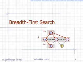
Maximum Flow by Incremental Breadth First Search
This work discusses a novel algorithm, Incremental Breadth-First Search (IBFS), for solving the maximum flow problem in directed graphs. IBFS enhances the existing strategies by performing nearly shortest-path augmentations, competing favorably with Boykov-Kolmogorov (BK) algorithms, often outperforming them in practice. We detail the three key phases of the IBFS algorithm—Growth, Augmentation, and Adoption—while ensuring a polynomial time guarantee. Applications in computer vision, such as image segmentation and stereo processing, underscore the practical relevance of efficient maximum flow algorithms.

Maximum Flow by Incremental Breadth First Search
E N D
Presentation Transcript
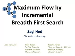
Maximum Flow byIncrementalBreadth First Search Sagi Hed Tel Aviv University Joint work with: Haim Kaplan Robert E. Tarjan Tel Aviv University Princeton University & HP Labs Renato F. Werneck Andrew V. Goldberg Microsoft Research Microsoft Research s
Maximum Flow • Input: graph G=(V,E), vertices s, t є V and capacity assignment c(e) for e є E • Output: flow function f satisfying -conservation: for every v≠s,t Σ(u,v)єE f(u,v) = Σ(v,u)єE f(v,u) capacity: for every e f(e) ≤ c(e)with maximal |f|=sum of flow out of s (into t) • Well studied problem • Equivalent to the Minimum s-t Cut problem • Solution methods:Augmenting Path (and blocking flow), Network Simplex, Push-Relabel
Push-Relabel • A different approach –Push vs. augment path, pre-flow vs. flow[Goldberg, Tarjan 88] • Some Push-Relabel bounds:O(mn2) Any active vertex selectionO(n3) FIFO active vertex selectionO(n2m½) Highest label active vertex selectionO(mn log(n2/m)) with dynamic trees • Push-Relabel considered the most efficient general-purpose solution in practice[Cherkassky, Goldberg 97]
Maximum Flowin Computer Vision • Minimum s-t cut very useful in the field of computer vision • Applications in image segmentation, stereo image processing, video transitioning… • Typical Process – • 2D or 3D images are converted to input graphs, where each vertex corresponds to a pixel • Minimum s-t cut on these graphs provides information on the original image(s)
Maximum Flowin Computer Vision • These graphs have specific structure • Regular low degree grids • Arc capacities: different models for grid arcs and s-t arcs
BK • Boykov and Kolmogorov developed an algorithm (BK) which is the fastest in practice on the vision instances[Boykov, Kolmogorov 04] • Used as the standard min-cut algorithm in computer vision • Usually outperforms Push-Relabel implementation by large factors • Problem: BK has no known polynomial time guarantee…Best bound is O(mnF) for integral capacities (F is the maximal flow value) • Indeed on some instances, BK performs poorly and is outperformed by Push-Relabel implementation
Our ContributionIBFS • We develop the IBFS algorithm –Incremental Breadth First Search • Has many similarities to BK and to Dinitz • However, performs shortest path or nearly shortest path augmentations • Competative in practice to BKUsually outperforms BK by small factors • Has a polynomial worst case time guaranteeO(mn2)
BK Overview • Grows trees S, T in the residual graph bi-directionally • We maintain a list of active nodes, from which the trees can grow active nodes t s s S T
BK Overview • When the trees meet, we augment flow • After an augmentation, we try to rebuild the trees active nodes t s s S T
BK Drill Down • Initially: S={s}, T={t}, active node list = {s,t} • Iterates between 3 phases:Growth, Augmentation, Adoption s s t S T
BK Drill Down • Growth: • Iterate through active node list and grow S,T • Add new vertices to the back of the active list (FIFO) s s s t t S T
BK Drill Down • Augment: • Discover other tree during growth => augment flow • Saturated tree arcs create orphan sub-trees s s Orphan t S T Orphan
BK Drill Down • Adoption: (symmetric for S and T) • Iterate over orphans and check potential parents • If an orphan finds a parent its entire subtree is reattached s t v
BK Drill Down • Adoption: • Checking a potential parent u: traverse the path from u to the root, no orphans on the path s t v
BK Drill Down • Adoption: Orphan v does not reconnect - • Remove v from tree and make children orphans • Make potential parents active • Make v inactive s t v
BK Drill Down • Continue Growth, Augmentation, Adoption • The trees are no longer neccesarily BFS trees • Augmenting paths are no longer neccesarily shortest • Growth alternates between S and T t s s S T
BK Drill Down • Termination: • No more active nodes (either in S or in T) • Maximum flow value is the total augmented flow t s s S T
IBFS Overview • We maintain S, T as BFS trees with heights ≈ Ds , Dt • Active nodes are on level Ds or Dt only • Augment on shortest (Ds+Dt+1) paths only (later nearly shortest paths) s s t S T Ds Dt
IBFS Overview • Vertex v has label ds(v) ≤ Ds+1 and a label dt(v) ≤ Dt+1 • ds(v) and dt(v), are the level of the tree v is in • ds(v) is meaningful if v ϵ S, dt(v) is meaningful if v ϵ T s s t S T Ds Dt
IBFS Drill Down • Initially: S={s}, T={t}, active node list = {s,t} • ds(s)=0, dt(t)=0, Ds=0, Dt=0 • As in BK, iterates between 3 phases:Growth, Augmentation, Adoption s s t S T
IBFS Drill Down • Growth: • Grow one complete level at a time, Ds++ or Dt++ • If u grows v, ds(v) = ds(u)+1 / dt(v) = dt(u)+1 • Can alternate forward/backward passes arbitrarily s s s t t S T dt=2 dt=1 dt=0 ds=0 ds=1 ds=2
IBFS Drill Down • Augment: • As in BK, • Discover other tree during growth => augment flow • Saturated tree arcs create orphan sub-trees s s Orphan t S T Orphan dt=2 dt=1 dt=0 ds=0 ds=1 ds=2
IBFS Drill Down • Adoption: (symmetric for S and T) • Iterate over orphans and check potential parents • If orphan v finds a parent u with dt(u)=dt(v)-1v’s subtree reconnects s t v dt=2 dt=1 dt=0
IBFS Drill Down • Adoption: Orphan v does not reconnect at same level – • Relabel(v): dt(v)=min{dt(u)|uϵT, (u,v) residual}+1parent(v) = argmin{...} • Make children orphans • Make v inactive v s t v dt=2 dt=1 dt=0
IBFS Drill Down • Adoption: (symmetric for S and T) • Remove v from T, if Relabel(v) does not find a parent • or Relabel(v) finds a parent u such that – • forward pass: dt(u) ≥ Dt backward pass: dt(u) ≥ Dt+1 s t v v dt=Dt=2 dt=1 dt=0
IBFS Drill Down • Adoption: (symmetric for S and T) • Orphan v may reconnect to an orphan subtree(its own or another) • If neccesary processed as an orphan again later s t v v dt=2 dt=1 dt=0
IBFS Drill Down • Continue Growth, Augmentation, Adoption • The trees are always maintained as BFS trees • Shortest augmenting paths = Ds+Dt+1 (proof soon) • Alternate between forward/backward passes s s t S T impossible Ds Dt
IBFS Drill Down • Termination: • Empty level (either in S or in T) • Maximum flow value is the total augmented flow t s s S T
IBFS vs. Dinitz • Basically a form of Dinitz • Bi-directional rather than uni-directional • Auxilary network for next passes prepared while processing current pass.Network not rebuilt from scratch every pass! s
IBFS Drill Down • Current Arc (time efficiency only) • Remeber where the last orphan parent scan stopped • When v is added to the tree, current arc = first arc • current_arc(v) ϵ {first_arc(v), (parent(v),v)}=> can be implemented with a bit s Current Arc s S
IBFS Correctness • Lemma 1: (symmetric for forward / backward passes) • If (u,v) is residual • During a forward pass –u in S, v not in S, ds(u) ≤ Ds => u active (ds(u)=Ds) • After we increase Ds until the next forward pass –u in S, v not in S => ds(u)=Ds Ds s s u u v u v S
IBFS Correctness • By Lemma 1, when the algorithm terminates there are no more residual augmenting paths=> the flow is maximal t s s S T
IBFS Time Bound • Definition: u,v in S, (u,v) is admissible:(u,v) is residual and ds(v) = ds(u)+1 • Algorithm Invariants: (symmetric for ds and dt) • Tree arcs are admissible • current arc of u precedes the first admissible arc to u • ds is a valid labeling: (u,v) residual => ds(v) ≤ ds(u)+1 • ds(v) never decreases s s
IBFS Time Bound • Algorithm Invariants Proof: • By induction on the algorithm steps. • Valid ds labeling (invariant 3):Growth step: By Lemma 1, there are no connections from lower levelsAugmentation: New residual arcs do not violate, by inductive assumption of admissible tree arcsAdoption: Orphan relabel does not break valid labeling (as in push-relabel) s
IBFS Time Bound • Conclusions from Algorithm Invariants:(not directly needed for analysis) • S and T are BFS trees:ds(v) = the distance from s to v in the residual graphdt(v) = the distance from v to t in the residual graph • We always augment on shortest paths in the residual graph s
IBFS Time Bound • Lemma 2: (symmetric for S and T) • After an orphan relabel on v in S, ds(v) increases. • If v is removed from S, then we consider the increased label the next time v is added to S. • Lemma 2 Proof: • Easy, except to avoidpathalogical case of adoption/growth s s v ds=0 ds=1 ds=2
IBFS Time Bound • Lemma 2 Proof: • Let U ≡ {u | u in S and (u,v) is residual} • Let ds’(v)=ds(v) at time of relabel(v) • By valid labeling and current arc invariants –If new_parent(v) ϵU=> ds(new_parent(v)) ≥ d’s(v)=> ds(v) = ds(new_parent(v))+1 ≥ d’s(v)+1 • By non-decreasing labels invariant, this is true at any future time s
IBFS Time Bound • Lemma 3: • IBFS runs in O(n2m) time • Lemma 3 Proof: (symmetric for S and T) • Note there are ≤ n-1 different values for ds(v) • GrowthWe charge the scan of arc (u,v) to ds(u)Each label charged by arc (u,v) at most once(u becomes inactive)Total: O(nm) s
IBFS Time Bound • Lemma 3 Proof continued: (symmetric for S and T) • AdoptionWe charge the scan of arc (u,v) (v orphan) to ds(v)Each label charged by arc (u,v) at most twice – • Once during scanning for a parent with label ds(v)-1(due to remembering the current arc) • Once during orphan relabel (by Lemma 2) Total: O(nm) s
IBFS Time Bound • Lemma 3 Proof continued: (symmetric for S and T) • AugmentationLet (u,v) be an arc saturated in the augmentation. • If (u,v) is a tree arc, we create an orphan – no more than charges made for adoption => O(nm) • If (u,v) is not a tree arc (u ϵ S, v ϵ T), we charge ds(u)Each label is charged by arc (u,v) at most once(u becomes inactive) => O(nm) Each augmentation takes O(n) time Total: O(n2m) □ s
IBFS Variants • Nearly Shortest Path • Vertices at level Ds in S and Dt in T are activated together • We grow both trees at the same time, intermittently • Augmenting paths are shortest or “shortest+1” • More similar to BK s s Ds+Dt+2 t S T dt=Dt=2 dt=1 dt=0 ds=0 ds=1 ds=Ds=2
IBFS Variants • Nearly Shortest Path • Passes are both forward and reverse at the same time • Correctness and running time are proved in the same way after applying the above rule • Proves best in practice • Used in our implementation and experiments s
IBFS Experiments • Ran on 37 computer vision instances, different families27 public benchmark [http://vision.csd.uwo.ca/maxflow-data/]10 our own creation [http://www.cs.tau.ac.il/~sagihed/ibfs/] • BK implementation available publicly [http://vision.csd.uwo.ca/code/] • We compare to a modified version of BK, with the same low level optimizations as our own (≈ 20% faster) • IBFS wins on 35 out of 372 different capacity versions of the instance “bone” • Factors are mostly modest. For few they are large. s
IBFS Experiments • Running Time (seconds) s
IBFS Experiments • Operation Counts • 4 operations counted: • Pushes – sum of augmentation lengths • Growth arc scans – number of arcs scanned during growth • Orphan arc scans – number of arcs scanned during adoption • Orphan traversal to root (BK) – number of arcs traverse to check the root of the potential parent’s tree • Growth and Orphan arc scans access arcs sequentially in memory • Pushes and Orphan traversal to root access arcs non-sequentially in memory s
IBFS Experiments • Operation Counts(per vertex) s
IBFS Experiments • On non computer-vision graph families [http://www.avglab.com/andrew/CATS/maxflow_synthetic.htm]IBFS outperforms BK, some by large factors • On these, standard Push-Relabel implementation outperforms both IBFS and BK. s
Summary • BK works well on computer vision problems in practice, but does not provide a polynomial run time guarantee • IBFS works as well in practice and provides a polynomial run time guarantee • IBFS operates similarly to BK, and can also be viewed as a bi-directional version of Dinitz where the auxiliary network is constantly recovered rather than rebuilt.
Open Question • Can you find a maximum-flow algorithm with a polynomial time bound, which is competitive in practice with both Push-Relabeland BK on all graph families?