Download

1 / 13
140 likes | 370 Views
Learn about Newton-Cotes integration formulas, the Trapezoidal Rule, Simpson’s Rules, and more for precise numerical calculations in engineering and mathematics. Discover how to apply these methods, like the Multiple-Application Trapezoidal Rule and Simpson’s 1/3 Rule, to improve accuracy in integrating functions. Explore examples, error estimates, and implementation in MATLAB.

E N D
~ Numerical Differentiation and Integration ~Newton-Cotes Integration FormulasChapter 21
Differentiation and Integration • Calculus is the mathematics of change. Since engineers continuously deal with systems and processes that change, calculus is an essential tool of engineering. • Standing at the heart of calculus are the concepts of:
Newton-Cotes Integration Formulas • Based on the strategy of replacing a complicated function or tabulated data with an approximating function that is easy to integrate: Zero order approximation First-order Second-order
The Trapezoidal Rule • Use a first order polynomial in approximating the function f(x) : • The area under this first order polynomial is an estimate of the integral of f(x) between a and b: Trapezoidal rule Error: where x lies somewhere in the interval from a to b
Example 21.1Single Application of the Trapezoidal Rulef(x) = 0.2 +25x – 200x2 + 675x3 – 900x4 + 400x5Integrate f(x) from a=0 to b=0.8 Solution:f(a)=f(0) = 0.2 and f(b)=f(0.8) = 0.232
The Multiple-Application Trapezoidal Rule • The accuracy can be improved by dividing the interval from a to b into a number of segments and applying the method to each segment. • The areas of individual segments are added to yield the integral for the entire interval. Using the trapezoidal rule, we get:
The Error Estimate for The Multiple-Application Trapezoidal Rule • Error estimate for one segment is given as: • An error for multiple-application trapezoidal rule can be obtained by summing the individual errors for each segment: Thus, if the number of segments is doubled, the truncation error will be quartered.
Simpson’s Rules • More accurate estimate of an integral is obtained if a high-order polynomial is used to connect the points. These formulas are called Simpson’s rules. Simpson’s 1/3 Rule: resultswhen a 2nd order Lagrange interpolating polynomial is used for f(x) a=x0x1 b=x2
The Multiple-Application Simpson’s 1/3 Rule • Just as the trapezoidal rule, Simpson’s rule can be improved by dividing the integration interval into a number of segments of equal width. • However, it is limited to cases where values are equispaced, there are an even number of segments and odd number of points.
Simpson’s 3/8 Rule Fit a 3rd order Lagrange interpolating polynomial to four points and integrate Simpson’s 1/3 and 3/8 rules can be applied in tandem to handle multiple applications with odd number of intervals
Newton-Cotes Closed Integration Formulas Same order, but Simpson’s 3/8 is more accurate In engineering practice, higher order (greater than 4-point) formulas are rarely used
Integration with Unequal Segments Using Trapezoidal Rule Example 21.7 which represents a relative error of e = 2.8% Data for f(x)= 0.2+25x-200x2+675x3-900x4+400x5
Compute Integrals Using MATLAB First, create a filecalledfx.mwhichcontains f(x): function y = fx(x) y = 0.2+25*x-200*x.^2+675*x.^3-900*x.^4+400*x.^5 ; Then, execute in thecommandwindow: >> Q=quad('fx', 0, 0.8) % true integral Q =1.6405 true value >> x=[0 .12 .22 .32 .36 .4 .44 .54 .64 .7 .8] >> y = fx(x) y = 0.200 1.309 1.305 1.743 2.074 2.456 2.843 3.507 3.181 2.363 0.232 >> Integral = trapz(x,y) % ortrapz(x, fx(x)) Integral =1.5948