Download
1 / 20
200 likes | 304 Views
14.4 Measures of Variation. CORD Math Mrs. Spitz Spring 2007. Objectives:. Calculate and interpret the range, quartiles, and interquartile range of a set of data. Assignment:. pp. 577-578 #1-24 all. Assignment. pp. 577-578 #1-24 all. Application.

E N D
14.4 Measures of Variation CORD Math Mrs. Spitz Spring 2007
Objectives: • Calculate and interpret the range, quartiles, and interquartile range of a set of data Assignment: • pp. 577-578 #1-24 all
Assignment • pp. 577-578 #1-24 all
Application • Pacquita Colon and Larry Neilson are two candidates for promotion to manager of sales at Fitright Shoes. In order to determine who should be promoted, the owner, Mr. Tarsel, looked at each person’s quarterly sales record for the past year. It’s on the next slide.
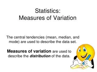
Application • After studying the data, Mr. Tarsel found that the mean of the quarterly sales was $30,500, the median was $30,600 and the mode was $31,000 for both Ms. Colon and Mr. Nielson. If he was to decide between the two, Mr. Tarsel needed to find more numbers to describe this data.
Application • The example shows that measures of central tendency may not give an accurate enough description of a set of data. Often, measures of variation, are also used to help describe the spread of the data. One of the most commonly used measures of variation is the range.
Definition of Range • The range of a set of data is the difference between the greatest and the least values of the set.
Ex. 1: Use the info in the table to determine the range in the quarterly sales for Ms. Colon and Mr. Nielson during the last two years. • Ms. Colon’s greatest quarterly sales were $31,000 and her least were $29,900. Therefore, the range is $31,000 - $29,900 or $1,100 • Mr. Nielson’s greatest quarterly sales were $33,200 and his least were $28,100. Therefore, the range is $33,200 - $28,100 or $5,100 • Based on this analysis, Ms. Colon’s sales are much more consistent, a quality Mr. Tarsel values. Therefore, Ms. Colon is promoted.
NOTE: • Another commonly used measure of variation is called the interquartile range. In a set of data, the quartiles are values that divide the data into four equal parts. The median of a set of data divides the data in half. The upper quartile (UQ) divides the upper half into two equal parts. The lower quartile (LQ) divides the lower half into two equal parts. The difference between the upper and lower quartile is the interquartile range.
Definition of the Interquartile Range • The difference between the upper quartile and the lower quartile of a set of data is called the interquartile range. It represents the middle half, or 50%, of the data in the set.
Ex. 2 • The Birch Corporation held its annual golf tournament for its employees. The scores for 18 holes were 88, 91, 102, 80, 115, 99, 101, 103, 105, 99, 95, 76, 105, and 112. Find the median, upper and lower quartiles, and the interquartile range for these scores.
First Step: • First, order the 15 scores. Then find the median. 70 80 88 91 95 99 99 101 102 103 105 105 112 115 139 { median
Second Step: • Find the median of the lower and upper quartiles. 70 80 88 91 95 99 99 101 102 103 105 105 112 115 139 { { { median lower quartile upper quartile The lower quartile is the median of the lower half of the data and the upper quartile is the median of the upper half. The interquartile range is 105 – 91 or 14. Therefore, the middle half, or 50%, or the golf scores vary by 14. The median divides the data in the data in half. The upper and lower quartiles divide each half into two parts.
NOTE: • In Example 2, one score, 139, is much greater than the others. In a set of data, a value that is much greater or much lower than the rest of the data is called an OUTLIER. An outlier is defined as any element of the set of data that is at least 1.5 interquartile ranges above the upper quartile or below the lower quartile.
NOTE: • To determine if 139 or any of the other numbers from Example 2 is an outlier, first multiply by 1.5 times the interquartile range, 14.
Ex. 3: The stem-and-leaf plot represents the number of shares of the 20 most active stocks that were bought and sold on the New York Stock Exchange. 4|0 represents 400,000,000 shares.
Ex. 3: The stem-and-leaf plot represents the number of shares of the 20 most active stocks that were bought and sold on the New York Stock Exchange. The brackets group the values in the lower half and the values in the upper half. What do the boxes contain? values used to find the lower and upper quartiles
Ex. 3: The stem-and-leaf plot represents the number of shares of the 20 most active stocks that were bought and sold on the New York Stock Exchange. The median is 26.
c. Find any outliers Since 46 > 41.75, 46 is an outlier. Since 11 < 41.75, 11 IS NOT an outlier.