Streaming Multigrid for Gradient-Domain Operations on Large Images

1. Streaming Multigridfor Gradient-Domain Operationson Large Images MishaKazhdan and Hugues Hoppe Johns Hopkins University Microsoft Research

2. Stitching Image Panoramas Gradient Domain Fix: Set seam-crossing gradients to zero. Different exposures  Seams in the panorama Courtesy of Uyttendaele

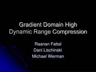
3. High Dynamic Range Compression Gradient Domain Fix: Amplify small gradients and dampen large ones. No single image exposes all the detail Medium Exposure Short Exposure Long Exposure Courtesy of Industrial Light & Magic Tone-Mapped Image

4. Gradient-Domain Image Processing Many image processing operations are easier to implement in the gradient-domain. GradientDomainOperator Image0  Grad0 GradientDomainOperator Image0 Grad0 Grad1 Solver  Grad1 Image1 Image1 Grad Image Image Solver Gradn Imagen  Gradn Grad Imagen   

5. Gradient-Domain Image Processing Many image processing operations are easier to implement in the gradient-domain. GradientDomainOperator Image0  Grad0 GradientDomainOperator Image0 Grad0 Grad1 Solver  Grad1 Image1 Image1 Grad Image Image Solver Gradn Imagen  Gradn Grad Imagen • [Horn ’74, Weiss ’01, Finlayson ’02, Agrawal ’05] • [Fattal ’02, Weyrich ’07] • [Perez ’03, Agarwala ’04, Jia ’06] • [Levin ’04, Agarwala ’07] • [McCann ’08] • Removing Lighting Effects • Range Compression • Image Compositing • Image Stitching • Image Authoring   

6. Gradient-Domain Image Processing Many image processing operations are easier to implement in the gradient-domain. GradientDomainOperator Image0  Grad0 GradientDomainOperator Image0 Grad1 Grad0 Solver  Grad1 Image1 Image1 Grad Image Image Solver Gradn Imagen  Grad Gradn Imagen • [Horn ’74, Weiss ’01, Finlayson ’02, Agrawal ’05] • [Fattal ’02, Weyrich ’07] • [Perez ’03, Agarwala ’04, Jia ’06] • [Levin ’04, Agarwala ’07] • [McCann ’08] • Removing Lighting Effects • Range Compression • Image Compositing • Image Stitching • Image Authoring   

7. Outline • Introduction • Solving for the Image • The Poisson Equation • Solving the Linear System • Choosing the System • Solving for Big Images • Results and Discussion

8. The Poisson Equation Gradient-domain processing requires fitting an image to local-difference constraints: ^ averaged g u f=div(g)

9. Gauss-Seidel Solvers Gradient-domain processing requires fitting an image to local-difference constraints. Iterative Algorithm: For each pixel (i,j) • Assume the rest of the pixel values are correct • Update u[i][j] to satisfy the Laplacian: ^ averaged u[i][j]  (Average of Neighbors) + f[i][j]

10. Gauss-Seidel Solvers This quickly solves for the high frequencies, but the low frequencies converge slowly. 2 Iteration Residual 2 Iterations 10 Iteration Residual 100 Iteration Residual 10 Iterations 100 Iterations Desired Solution

11. Multigrid Solvers V-Cycle Algorithm: The process is recursed for the low-res problem. Refine the high-res image Perform a few updates on the high-res image Compute the residual constraints Down-sample, solve, and up-sample Sum the low-res and high-res results + Desired Best-Guess Best-Guess Iterated Iterated - Desired Solved Residual Up-Sampled

12. Outline • Introduction • Solving for the Image • Choosing the System • Solving for Big Images • Results and Discussion

13. Choosing the System The choice depends on the interpretation of pixels as elements of a continuous function. Pixel values 0th-order interpretation 1st-order interpretation 2nd-order interpretation 3rd-order interpretation Elements

14. Choosing the System Implementing Up-/Down-Sampling: The nesting of the elements determines the transition between the levels of the solver. 1 1 1 0th-order elements 1st-order elements 2nd-order elements 3rd-order elements 3/4 3/4 3/4 1/2 1/2 1/2 1/2 1/4 1/4 1/8 1/8

15. Choosing the System Defining the Laplacian: The neighborhood of the Laplacian is defined by the element overlap. 0th-order elements 1st-order elements 2nd-order elements 3rd-order elements Undefined 1-Ring Average 2-Ring Average 3-Ring Average

16. Second-Order Elements Which order elementconverges fastest to anaccurate solution? 1st-order error 2nd-order error Original Image Image Gradients 3rd-order error

17. Second-Order Elements Spectral Analysis of Convergence: The eigenvalues of the multigrid operator determine how efficiently the residual is dampened. G.S Update G.S Update Up-Sample Down-Sample G.S Update Two-Grid Operator

18. Outline • Introduction • Solving for the Image • Choosing the System • Solving for Big Images • Naïve Out-of-Core Multigrid • Temporal Blocking • Interleaved Multilevel Streaming • Results and Discussion

19. Naïve Out-of-Core Multigrid Components of the solver: • Gauss-Seidel updates • Down-sampling • Up-sampling The multigrid solvercan be streamed byadvancing a fixed-size window. Local data access On Disk In Memory

20. Naïve Out-of-Core Multigrid The large linear system can be solved by streaming each step of the V-cycle. Constraints G.S. Update Solution G.S. Update k k Residual Up-Sample Down-Sample G.S. Update G.S. Update k k Residual Up-Sample k Gauss-Seidel Updates2(k+2) Streaming Passes Down-Sample Disk Streaming Low-Res Solve

21. Temporal Blocking A pixel can be updated for the kth time only if all other pixels have been updated k-1 times. neighbor

22. Temporal Blocking A pixel can be updated for the kth time only if all other pixels have been updated k-1 times. neighbor Window 2 1  2 0 0  1 1  2 0 0  1 0  1 1  2 0 0 0  1 0 0  1 0 2nd-order elements 0 k=2 Gauss-Seidel Updates

23. Temporal Blocking A pixel can be updated for the kth time only if all other pixels have been updated k-1 times. neighbor Constraints G.S. Update Solution G.S. Update Residual Up-Sample Down-Sample G.S. Update G.S. Update Residual Up-Sample Down-Sample Disk Streaming Low-Res Solve

24. Interleaved Multilevel Streaming Processing at one level is buffered for the next. piped into

25. Interleaved Multilevel Streaming Processing at one level is buffered for the next. High-Resolution Low-Resolution piped into Residual ¼ ¼ ¼ ¾ ¾ ¾ 0 0  1 0 0  1 2 1  2 ¾ ¾ ¾ 0 2 1  2 0  1 ¼ ¼ ¼ 0 0 2 0  1 1  2 0 0  1 1  2 2 0 0 1 2 0  1 0 0  1 1 2 3/4 3/4 0 1 2 0  1 0 0  1 1 2 1/4 0 0  1 1 2 1/4 0 0  1 0 0  1 0 0 2nd-order elements

26. Interleaved Multilevel Streaming Processing at one level is buffered for the next. Streaming Pass 1 Streaming Pass 2 piped into Constraints G.S. Update Solution G.S. Update Residual Up-Sample Down-Sample Globality of the Poisson equation  Two streaming passes is optimal G.S. Update G.S. Update Residual Up-Sample Down-Sample Memory Streaming Disk Streaming Disk Streaming Low-Res Solve

27. Streaming through the Gradient-Domain For gradient-domain operators that are local, processing only takes two streaming passes. +1 streaming pass for each additional V-cycle. Update u0 g0  Op Pass 1 Pass 2 Pass 3 u1 g1  f g  Update … u u … Update Update … un gn  Update Update Update Update Solve Memory Streaming Disk Streaming Solve

28. Outline • Introduction • Solving for the Image • Choosing the System • Solving for Big Images • Results and Discussion

29. Stitching Big Images • Agarwala ’07: • A high-res solution is only required near the seams, so solve over an adapted quadtree. Courtesy of Agarwala

30. Stitching Results Rainier: 10,9602,096 Beynac: 6,0461,920 Edinburgh: 16,9502,956 Redrock: 19,5884,457 Courtesy of Agarwala and Curless

31. Tone-Mapping Results Bring out subtle details by amplifying small gradients and dampening large ones.

32. Large Image Results St James: • Stitched from 643 photographs • Contains 3.3 billion (88,309 x 37,842) pixels Stitched Memory: 408 MB Time: 1:27:50 Max Error [0,256): 0.15 Tone-Mapped Memory: 224 MB Time: 45:10 Max Error [0,256): 0.5 Courtesy of Uyttendaele

33. Large Image Results St James: • Peak Memory: 408 MB • Solver Time: 1:27:50 Total disk I/O: • Down-Sampling • Read in the gradient constraints: 40 GB • Write out solution and Laplacian: 53 GB • Up-Sampling • Read in solution and Laplacian: 53 GB • Write out the image: 20 GB 53GB in-core 1:19:02 I/O Time Courtesy of Uyttendaele

34. Summary Streaming multigrid for big image processing: • 2nd order elements • Temporal blocking • Interleaved streaming Issues addressed in the paper: • Integration with finite-differences • Setting the average color • Non power-of-two images Accurate solution in two streaming passes

35. Issues for Future Work • Non-trivial boundaries and constraints? e.g. cut-and-paste, matting • Adaptive weighting? e.g. local tone adjustment • Extensions to higher dimensions? for incompressible fluid simulation • Less I/O in the streaming passes? on-the-fly compression • Really big images? parallelized and distributed solvers

36. Acknowledgments Datasets: AseemAgarwala Brian Curless Matt Uyttendaele Discussions and Ideas: KetanDalal Rick Szeliski Bill Bolosky Ann Wolverton CAVGRAPH Reviewers SIGGRAPH Reviewers

37. Thank You! Code & Images @ http://www.cs.jhu.edu/~misha/Code/SMG

39. General Temporal Blocking To perform k updates: Updating the 3rd row from front,The row two behind that,The row two behind that, k Window … 2  3 0 3 1  2 0  1 2  3 1  2 0 0  1 2  3 0  1 1  2 0 1  2 0 0  1 1  2 0 0  1 0  1 0 0  1 0 0 0 k=3 Gauss-Seidel Updates

40. General Temporal Blocking To perform k updates: Updating the 3rd row from front,The row two behind that,The row two behind that, … (d+1)-st with d-th order elements ^ d k d 3 2  3 2  3 1  2 1  2 Window 0  1 0  1 0 0 k=3 Gauss-Seidel Updates

41. Finite Differences to Finite Elements The derivative of a d-th order element is the difference of elements of order d-1. 1st-order Element Finite Differences Differentiation Coefficients of Derivative Elements 0th-order Elements

42. Second-Order Elements Which order elementconverges fastest to anaccurate solution? 1st-order error 2nd-order error Original Image Image Gradients 1/256 1/256 3rd-order error