Download

1 / 43
430 likes | 458 Views
Explore non-linear regression modeling using the trees data frame in R to predict timber volume based on tree girth, with graphical analysis and model comparisons for better insights.

E N D
The data frame trees is made available in R with >data(trees) These record the girth in inches, height in feet and volume of timber in cubic feet of each of a sample of 31 felled black cherry trees in Allegheny National Forest, Pennsylvania. Note that girth is the diameter of the tree (in inches) measured at 4 ft 6 in above the ground.
We treat volume as the (continuous) response variable y and seek a reasonable model describing its distribution conditional first on the explanatory variable girth (we will call this x). This might be a first step to prediction of volume based on further observations of the explanatory variables.
Observation of the graph leads us to first try out whether there may be a linear dependence here. Thus the relationship is approximately y=a+bx+є, for some constants a and b We will use R to find a and b, their standard errors and the residuals.
The fitted model is volume = −36.9 + 5.07 × girth + residual i.e. y = −36.9 + 5.07x (+ residual) To check its validity, first look at the standard errors
The standard errors of both a and b are low in comparison with the actual values and the p-values associated with the coefficients show that neither of these may reasonably be taken as zero. Thus there is evidence that the model is appropriate.
Some measure of the success of the fitted model is also given by the residual standard error. For a good fit this should be small in relation to the variation in the response variable itself.
However, a full examination of the residuals, and of the nature of any further dependence they may have on the explanatory variables, is to be preferred to reliance on any single number. All this will require graphical analysis, the results of which follow.
There is a slight evidence of non random behaviour in the residuals with perhaps the hint of a quadratic curve. We now adapt the model.
The residuals from Model 1 show some further, perhaps quadratic, dependence on the explanatory variable girth, so we try introducing a nonlinear term. We consider the model volume = a + b1 × girth + b2× (girth)2 + resid The relevant R commands, and associated output, are now >model2 = lm(Volume~Girth+I(Girth^2)) > summary(model.2)
The fitted model is therefore volume = 10.8 − 2.09 × girth + 0.255 × (girth)2 + residual.
Consider now the graphs produced by the following commands. > plot(Volume~Girth) > lines(fitted(model2)~Girth) > plot(residuals(model2)~Girth, ylab="residuals from Model 2")
It is clear that these residuals are both smaller than those from Model 1 and show no further obvious dependence on the explanatory variable girth. Further the very small p-value (0.00015) associated with the coefficient b2 shows that this cannot reasonably be set equal to zero, so that Model 2 is considerably more successful than Model 1.
Note also that the residual standard error in Model 2 is 3.335 whilst in Model 1 it is 4.252. Further Analysis: On physical grounds, we might also consider the simpler model Volume = b2 × (Girth)2 + Residual For extra justification look at this R output
The R code to fit this model, and brief summary output, are: > model3 = lm(Volume ~ I(Girth^2) - 1) > summary(model3)
We might now ask if we can find a model with both explanatory variables height and girth. Physical considerations suggest that we should explore the very simple model Volume = b1 × height × (girth)2 + This is basically the formula for the volume of a cylinder.
So the equation is: Volume = 0.002108 × height × (girth)2 +
The residuals are considerably smaller than those from any of the previous models considered. Further graphical analysis fails to reveal any further obvious dependence on either of the explanatory variable girth or height. Further analysis also shows that inclusion of a constant term in the model does not significantly improve the fit. Model 4 is thus the most satisfactory of those models considered for the data.
However, this is regression “through the origin” so it may be more satisfactory to rewrite Model 4 as volume = b1 + height × (girth)2
so that b1 can then just be regarded as the mean of the observations of volume height × (girth)2 recall that is assumed to have location measure (here mean) 0.
Adding an extra point: > ynew=c(y,12) > x1new=c(x1,20) > x2new=c(x2,100) > multregressnew=lm(ynew~x1new+x2new)