Functional Programming
Functional Programming. Universitatea Politehnica Bucuresti 2008-2009 Adina Magda Florea http://aimas.cs.pub.ro/fp_09. L1 – Course content. Introduction, programming paradigms, basic concepts Introduction to Scheme Expressions, types, and functions Lists Programming techniques


Functional Programming
E N D
Presentation Transcript
Functional Programming Universitatea Politehnica Bucuresti2008-2009 Adina Magda Florea http://aimas.cs.pub.ro/fp_09
L1 – Course content • Introduction, programming paradigms, basic concepts • Introduction to Scheme • Expressions, types, and functions • Lists • Programming techniques • Name binding, recursion, iterations, and continuations • Introduction to Haskell • Problem solving paradigms in FP
Course materials Scheme resources • Almost all you want to know and find about Scheme http://www.schemers.org/ • Development and execution environment http://www.drscheme.org/ • Books and research articles on Scheme http://library.readscheme.org/page2.html • R. Kent DybvigThe Scheme Programming Language, Second Edition – online book http://www.scheme.com/tspl2d/index.html Haskell http://www.haskell.org/ • Haskell language design http://haskell.readscheme.org/lang_sem.html
Requirements • Laboratory: min 6 • Laboratory assignments • Homeworks • Final exam Grading • Laboratory assignments and homewwork 50% • Final exam 50%
Lecture No. 1 • Introduction to FP • Mathematical functions • LISP • Introduction to Scheme
1. Introduction to FP • The design of the imperative languages is based directly on the von Neumann architecture • Efficiency is the primary concern, rather than the suitability of the language for software development • The design of the functional languages is based on mathematical functions • A solid theoretical basis that is also closer to the user, but relatively unconcerned with the architecture of the machines on which programs will run
1.1 Principles of FP • treats computation as evaluation of mathematical functions (and avoids state) • data and programs are represented in the same way • functions as first-class values – higher-order functions: functions that operate on, or create, other functions – functions as components of data structures • lamda calculus provides a theoretical framework for describing functions and their evaluation • it is a mathematical abstraction rather than a programming language
1.2 History • lambda calculus (Church, 1932) • simply typed lambda calculus (Church, 1940) • lambda calculus as prog. lang. (McCarthy(?), 1960, Landin 1965) • polymorphic types (Girard, Reynolds, early 70s) • algebraic types ( Burstall & Landin, 1969) • type inference (Hindley, 1969, Milner, mid 70s) • lazy evaluation (Wadsworth, early 70s) • Equational definitions Miranda 80s • Type classes Haskell 1990s
1.3 Varieties of FP languages • typed (ML, Haskell) vs untyped (Scheme, Erlang) • Pure vs Impure • impure have state and imperative features • pure have no side effects, “referential transparency” • Strict vs Lazy evaluation
1.4 Declarative style of programming • Declarative Style of programming - emphasis is placed on describing what a program should do rather than prescribing how it should do it. • Functional programming - good illustration of the declarative style of programming. • A program is viewed as a function from input to output. • Logic programming – another paradigm • A program is viewed as a collection of logical rules and facts (a knowledge-based system). Using logical reasoning, the computer system can derive new facts from existing ones.
1.5 Functional style of programming • A computing system is viewed as a function which takes input and delivers output. • The function transforms the input into output . • Functions are the basic building blocks from which programs are constructed. • The definition of each function specifies what the function does. • It describes the relationship between the input and the output of the function.
Examples • Describing a game as a function • Text processing • Text processing: translation • Compiler
1.6 Why functional programming • Functional programming languages are carefully designed to support problem solving. • There are many features in these languages which help the user to design clear, concise, abstract, modular, correct and reusable solutions to problems. • The functional Style of Programming allows the formulation of solutions to problems to be as easy, clear, and intuitive as possible. • Since any functional program is typically built by combining well understood simpler functions, the functional style naturally enforces modularity.
Why functional programming • Programs are easy to write because the system relieves the user from dealing with many tedious implementation considerations such as memory management, variable declaration, etc . • Programs are concise (typically about 1/10 of the size of a program in non-FPL) • Programs are easy to understand because functional programs have nice mathematical properties (unlike imperative programs) . • Functional programs are referentially transparent , that is, if a variable is set to be a certain value in a program; this value cannot be changed again. That is, there is no assignment but only a true mathematical equality.
Why functional programming • Programs are easy to reason about because functional programs are just mathematical functions; • hence, we can prove or disprove claims about our programs using familiar mathematical methods and ordinary proof techniques (such as those encountered in high school Algebra). • For example we can always replace the left hand side of a function definition by the corresponding right hand side.
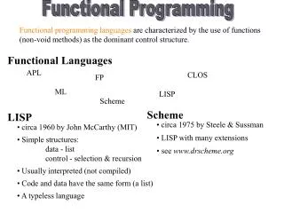
1.7 Examples of FP languages • Lisp (1960, the first functional language….dinosaur, has no type system) • Hope (1970s an equational fp language) • ML (1970s introduced Polymorphic typing systems) • Scheme (1975, static scoping) • Miranda (1980s equational definitions, polymorphic typing • Haskell (introduced in 1990, all the benefits of above + facilities for programming in the large.) • Erlang (1995 - a general-purpose concurrent programming language and runtime system, introduced by Ericsson) • The sequential subset of Erlang is a functional language, with dynamic typing.
2. Mathematical functions • Def: A mathematical function is a mapping of members of one set, called the domain set, to another set, called the range set • A lambda expression specifies the parameter(s) and the mapping of a function in the following form (x) x * x * x for the function cube (x) = x * x * x
Mathematical functions • Lambda expressions describe nameless functions • Lambda expressions are applied to parameter(s) by placing the parameter(s) after the expression e.g. ((x) x * x * x)(3) which evaluates to 27
Mathematical functions • Functional Forms • Def: A higher-order function, or functional form, is one that either takes functions as parameters or yields a function as its result, or both
Functional forms 1. Function Composition • A functional form that takes two functions as parameters and yields a function whose value is the first actual parameter function applied to the application of the second Form: h f ° g which means h (x) f ( g ( x)) For f (x) x * x * x and g (x) x + 3, h f ° g yields (x + 3)* (x + 3)* (x + 3)
Functional forms 2. Construction • A functional form that takes a list of functions as parameters and yields a list of the results of applying each of its parameter functions to a given parameter Form: [f, g] For f (x) x * x * x and g (x) x + 3, [f, g] (4) yields (64, 7)
Functional forms 3. Apply-to-all • A functional form that takes a single function as a parameter and yields a list of values obtained by applying the given function to each element of a list of parameters Form: For h (x) x * x * x ( h, (3, 2, 4)) yields (27, 8, 64)
3. LISP • Lambda notation is used to specify functions and function definitions. Function applications and data have the same form. e.g., If the list (A B C) is interpreted as data it is a simple list of three atoms, A, B, and C If it is interpreted as a function application, it means that the function named A is applied to the two parameters, B and C • The first LISP interpreter appeared only as a demonstration of the universality of the computational capabilities of the notation
4. Introduction to Scheme • A mid-1970s dialect of LISP, designed to be a cleaner, more modern, and simpler version than the contemporary dialects of LISP • Invented by Guy Lewis Steele Jr. and Gerald Jay Sussman • Emerged from MIT • Originally called Schemer • Shortened to Scheme because of a 6 character limitation on file names
Introduction to Scheme • Designed to have very few regular constructs which compose well to support a variety of programming styles • Functional, object-oriented, and imperative • All data type are equal • What one can do to one data type, one can do to all data types
Introduction to Scheme • Uses only static scoping • Functions are first-class entities • They can be the values of expressions and elements of lists • They can be assigned to variables and passed as parameters
Introduction to Scheme • Primitive Functions 1. Arithmetic:+, -, *, /, ABS, SQRT, REMAINDER, MIN, MAX e.g., (+ 5 2) yields 7
Introduction to Scheme 2.QUOTE -takes one parameter; returns the parameter without evaluation • QUOTE is required because the Scheme interpreter, named EVAL, always evaluates parameters to function applications before applying the function. QUOTE is used to avoid parameter evaluation when it is not appropriate • QUOTE can be abbreviated with the apostrophe prefix operator e.g., '(A B) is equivalent to (QUOTE (A B))
Introduction to Scheme 3. CAR takes a list parameter; returns the first element of that list e.g., (CAR '(A B C)) yields A (CAR '((A B) C D)) yields (A B) 4. CDR takes a list parameter; returns the list after removing its first element e.g., (CDR '(A B C)) yields (B C) (CDR '((A B) C D)) yields (C D)
Introduction to Scheme 5. CONS takes two parameters, the first of which can be either an atom or a list and the second of which is a list; returns a new list that includes the first parameter as its first element and the second parameter as the remainder of its result e.g., (CONS 'A '(B C)) returns (A B C)
Introduction to Scheme 6. LIST - takes any number of parameters; returns a list with the parameters as elements
Introduction to Scheme • Lambda Expressions • Form is based on notation e.g., (LAMBDA (L) (CAR (CAR L))) L is called a bound variable • Lambda expressions can be applied e.g., ((LAMBDA (L) (CAR (CAR L))) '((A B) C D))
Introduction to Scheme • A Function for Constructing Functions DEFINE - Two forms: 1. To bind a symbol to an expression e.g., (DEFINE pi 3.141593) (DEFINE two_pi (* 2 pi))
Introduction to Scheme 2. To bind names to lambda expressions e.g., (DEFINE (cube x) (* x x x)) Example use: (cube 4)
Introduction to Scheme • Evaluation process (for normal functions): 1. Parameters are evaluated, in no particular order 2. The values of the parameters are substituted into the function body 3. The function body is evaluated 4. The value of the last expression in the body is the value of the function (Special forms use a different evaluation process)
Introduction to Scheme • Example: (DEFINE (square x) (* x x)) (DEFINE (hypotenuse side1 side1) (SQRT (+ (square side1) (square side2))) )
Introduction to Scheme • Example: (define (list-sum lst) (cond ((null? lst) 0) ((pair? (car lst)) (+(list-sum (car lst)) (list-sum (cdr lst)))) (else (+ (car lst) (list-sum (cdr lst))))))
Some conventions Naming Conventions • A predicate is a procedure that always returns a boolean value (#t or #f). By convention, predicates usually have names that end in `?'. • A mutation procedure is a procedure that alters a data structure. By convention, mutation procedures usually have names that end in `!'.
Cases Uppercase and Lowercase • Scheme doesn't distinguish uppercase and lowercase forms of a letter except within character and string constants; in other words, Scheme is case-insensitive. • For example, Foo is the same identifier as FOO, but 'a' and 'A' are different characters.
Predicate functions • Predicate Functions: (#t is true and #f or ()is false) 1. EQ? takes two symbolic parameters; it returns #T if both parameters are atoms and the two are the same e.g., (EQ? 'A 'A) yields #t (EQ? 'A '(A B)) yields () • Note that if EQ? is called with list parameters, the result is not reliable • Also, EQ? does not work for numeric atoms
Predicate functions • Predicate Functions: 2. LIST? takes one parameter; it returns #T if the parameter is a list; otherwise() 3. NULL? takes one parameter; it returns #T if the parameter is the empty list; otherwise() Note that NULL? returns #T if the parameter is() 4. Numeric Predicate Functions =, <>, >, <, >=, <=, EVEN?, ODD?, ZERO?, NEGATIVE?
Control flow • Control Flow 1. Selection- the special form, IF (IF predicate then_exp else_exp) e.g., (IF (<> count 0) (/ sum count) 0 )
Control flow • Control Flow 2. Multiple Selection - the special form, COND General form: (COND (predicate_1 expr {expr}) (predicate_1 expr {expr}) ... (predicate_1 expr {expr}) (ELSE expr {expr}) ) Returns the value of the last expr in the first pair whose predicate evaluates to true
Example (DEFINE (compare x y) (COND ((> x y) (DISPLAY “x is greater than y”)) ((< x y) (DISPLAY “y is greater than x”)) (ELSE (DISPLAY “x and y are equal”)) ) )
Example 1. member - takes an atom and a simple list; returns #T if the atom is in the list; () otherwise (DEFINE (member atm lis) (COND ((NULL? lis) '()) ((EQ? atm (CAR lis)) #T) ((ELSE (member atm (CDR lis))) ))
Example 2. equalsimp - takes two simple lists as parameters; returns #T if the two simple lists are equal; () otherwise (DEFINE (equalsimp lis1 lis2) (COND ((NULL? lis1) (NULL? lis2)) ((NULL? lis2) '()) ((EQ? (CAR lis1) (CAR lis2)) (equalsimp(CDR lis1)(CDR lis2))) (ELSE '()) ))
Example 3. equal - takes two general lists as parameters; returns #T if the two lists are equal; ()otherwise (DEFINE (equal lis1 lis2) (COND ((NOT (LIST? lis1))(EQ? lis1 lis2)) ((NOT (LIST? lis2)) '()) ((NULL? lis1) (NULL? lis2)) ((NULL? lis2) '()) ((equal (CAR lis1) (CAR lis2)) (equal (CDR lis1) (CDR lis2))) (ELSE '()) ))
Example 4. append - takes two lists as parameters; returns the first parameter list with the elements of the second parameter list appended at the end (DEFINE (append lis1 lis2) (COND ((NULL? lis1) lis2) (ELSE (CONS (CAR lis1) (append (CDR lis1) lis2))) ))