Parallel Scalability
Parallel Scalability . CS 420 Fall 2012 Osman Sarood. How faster can we run?. Suppose we have this serial problem with 12 tasks. How fast can we run given 3 processors?. Running in parallel. Execution time reduces from 12 secs to 4 secs !. Load imbalance .


Parallel Scalability
E N D
Presentation Transcript
Parallel Scalability CS 420 Fall 2012 Osman Sarood
How faster can we run? • Suppose we have this serial problem with 12 tasks. How fast can we run given 3 processors?
Running in parallel • Execution time reduces from 12 secs to 4 secs!
Load imbalance • What if all processors can’t execute tasks with the same speed? • Load imbalance (ending parts for W2 and W3)
Dependence amongst tasks • What if tasks 3, 7 and 11 are dependent? • Execution time increases from 4 to 6!
Scalability • How much faster can a given problem be solved with N workers instead of one? • How much more work can be done with N workers instead of one? • What impact for the communication requirements of the parallel application have on performance? • What fraction of the resources is actually used productively for solving the problem?
Scalability • Simple model s: is the serial part p: is the parallel part • Why serial part? • Algorithm limitations: dependencies • Bottlenecks: shared resources • Startup overhead: starting a parallel program • Communication: interacting with others workers
Scaling • Strong Scaling: Keeping the problem size fixed and pushing in more workers or processors • Goal: Minimize time to solution for a given problem • Weak Scaling: Keeping the work per worker fixed and adding more workers/processors (the overall problem size increases) • Goal: solve the larger problems
Strong Scaling • Work done • Single worker runtime: • Same problem in parallel on N workers takes:
Weak Scaling • Work done • Single worker runtime: • Same problem in parallel on N workers takes:
Performance: Strong Scaling • Performance = work / time • Strong scaling: • Serial performance: • Parallel performance: • Speedup: The same!
Example: Strong Scaling • s: 0.1, p: 0.9, N: 1000 |s: 0.9, p: 0.1, N: 1000 • Strong scaling: • Serial performance: • 1 |1 • Parallel performance and speedup: 9.91 |1.11
Strong Scaling changing “work” • Work: p ( only the parallelizable part) • Strong scaling: • Serial performance: since • Parallel performance: • Speedup: Differ by factor of ‘p’ But speedup is the same
Example: Strong Scaling • s: 0.1, p: 0.9, N: 1000 |s: 0.9, p: 0.1, N: 1000 • Strong scaling: • Serial performance: 0.9 | 0.1 • Parallel performance: 8.9 | 0.11 • Speedup: • 9.9 | 1.11
Performance: Weak Scaling • Weak scaling: • Serial performance: • Parallel performance:
Gustafson’s law • In case we recover Amdahl’s law. • For and when N is large, • is linear in • hence, we can cross Amdahl’s law and get unlimited performance!
Gustafson’s law • In the case • Speedup is linear in N
Weak Scaling changing “work” • Work: p ( only the parallelizable part) • Weak scaling: • Serial performance: • Parallel performance: • Speedup: Differ by factor of ‘p’
Scalability: Weak Scaling • For , • Linear in with a slope of 1 • Makes us believer that all is well and application scales perfectly • Remember previously, in Gustafson’s equation, it had a slope of (1-s)<1
Parallel Efficiency • How effectively CPU computational power can be used in a parallel program.
Effect of • For , (is there any significance of it?) • As N increases, decreases to 0 • For , • Efficiency reaches a limit of 1-s=p. Weak scaling enables us to use at least a certain fraction of CPU power even when N is large • The more CPUs are used, the more CPU cycles are wasted (What do you understand by it?)
Changing “work” • If work is defined as only the parallel part ‘p’ • For , we get • Implied perfect scalability! • And no CPU cycles are wasted! • Is that true?
Example • Some application has flops only in the parallel region • s: 0.9 and p: 0.1 • 4 CPUs spend 90% idle! • MFLOPs rate a factor of N higher than serial case
Serial performance and strong scalability • Ran the same code on 2 different architectures • Single thread performance is the same • Serial fraction `s’ much smaller on arch2 due to greater memory bandwidth
Serial performance and strong scalability • Scalar optimizations (studied earlier) should be done in serial or parallel parts? • Assuming serial part can be accelerated by parallel performance becomes: • In case parallel part is improved parallel performance becomes:
Serial performance and strong scalability • When does optimizing the serial part pays off more than optimizing the parallel part: • Does not depend on • If , it pays off to optimize parallel region as serial optimization would be beneficial after a very large value of N.
Are these simple models enough? • Amdahl’s law for strong scaling • Gustafson’s law for weak scaling • Problems with these models? • Communication • More memory (affects both strong and weak scaling?) • More cache (affects both strong and weak scaling?)
Accounting communication • Where do we account for communication? • Do we increase the work done? • Do we increase the execution time? • It should affect the parallel execution time only as it doesn’t affect the work done (its not ‘useful’ work)
Weak scaling: Speedup • Speedup reduces due to communication: • What is ? • It depends on the type of network • Blocking • Non blocking • Depends on (latency) and (time taken to transmit depending on number of bytes ‘n’ and bandwidth ‘B’
Effects of communication on Speedup • Blocking network: • is dependent of N since network is blocking and one proc can send msg at a time. • Speedup goes -> 0 for large N due to communication bottleneck
Effects of communication on Speedup • non-Blocking network, constant size message: • is independent of N since network is nonblocking and procs can send msg at the same time. • Speedup settles to a lower value than what it was without incorporating communication • Better than blocking case
Effects of communication on Speedup • non-Blocking network with ghost layer communication: • is inversely dependent on N. Why? • Speedup settles to a lower value than what it was without incorporating communication • Better than non-blocking constant comm. cost.
Effects of communication on Speedup • non-Blocking network with ghost layer communication, : • is independent of N (constant) since the problem size also grows linearly with N • Speedup is linear as this is weak scaling • But less than what it was w/o communication
Predicted Scalability for different models • Speedup for: • Weak scaling keeps on increasing linearly • Strong scaling is projectile and hits zero for large N • Other models lie in between • All strong scaling models less than Amdahl’s
Scaling baseline • How do we normalize the results for determining speedup? • Speedup using model slide 30
Scaling baseline (main figure) • The main figure shows higher serial part: 0.2 with no effect from communication k: 0 • The actual points are way from the prediction (for small core count) • Main figure is normalized using single core performance
Right smaller figure • Change baseline from per core to per node • Almost a perfect fit! • Serial fraction s:0.01, comm k=0.05 • Much more dependence on comm!
Left smaller figure • Changes baseline to per core but only shows whats going on inside a node • Bad speedup moving from 1core->2core (due to use of same socket) • Sudden jump in speedup from 2-4 cores (an additional socket)
Scaling baseline takeaway Scaling behavior for inter and intra node cases should be studied seperately
Load imbalance • What is load imbalance? Speeder Lagger
Load imbalance • Both speeder and laggers are bad. • Which one is worse? • A few laggers (majority speeders) • A few speeders (majority laggers) • How much time is spent idle?
Reasons for load imbalance (1) • The method chosen for distributing work among the workers may not be compatiblewith the structure of the problem • JDS sparse matrix-vector multiply • Allocate equal number of row to all procs • Some rows might have significantly more non-zeros compared to others
Reasons for load imbalance (2) • It may notbe known at compile time how much time a “chunk” of work actually takes • Applications having the concept of convergence. Each chunk needs to execute until it converges. You can’t determine the number of instructions to convergence before hand (mostly)
Reasons for load imbalance (3) • There may be a coarse granularity to the problem, limiting the available parallelism. • This happens usually when the number of workers is not significantlysmaller than the number of work packages. • Imagine having 10000 tasks with 6000 processors
Reasons for load imbalance (4) • If a worker has to wait forresources like, e.g., I/O or communication devices. • overhead of this kind is often statistical in nature,causing erratic load imbalance behavior • How can we remedy such problems? • For communication we can try and overlap communication and computation
Reasons for load imbalance (5) • Dynamically changing workload • Adaptive Mesh Refinement, Molecular dynamics • Workload might be balanced to start with but can change gradually over time • Adapting to such dynamic workload is not easy for MPI programmers
Charm++ • Based on object based over-decomposition • Programmer can think in terms of objects instead of processors. • Offers automatic: • dynamic load balancing • Fault tolerance • Energy/Power efficient HPC applications • More to come in later lectures
OS Jitter • Interference from OS • Causes load imbalance • Statistical in nature e.g. 1 out of 4 four processors will get OS interference in 1 sec
OS Jitter on larger machines • OS jitter much more harmful in larger machines
OS Jitter synchronization • Synchronize processors so that OS jitters happen roughly at the same time for all processors • Difficult to do (requires significant OS hacking)