Precipitation and Cloud Structure in Midlatitude Cyclones

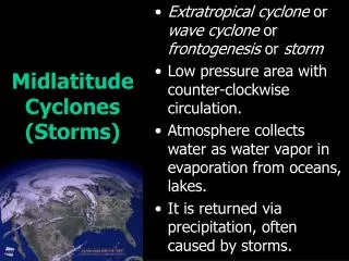
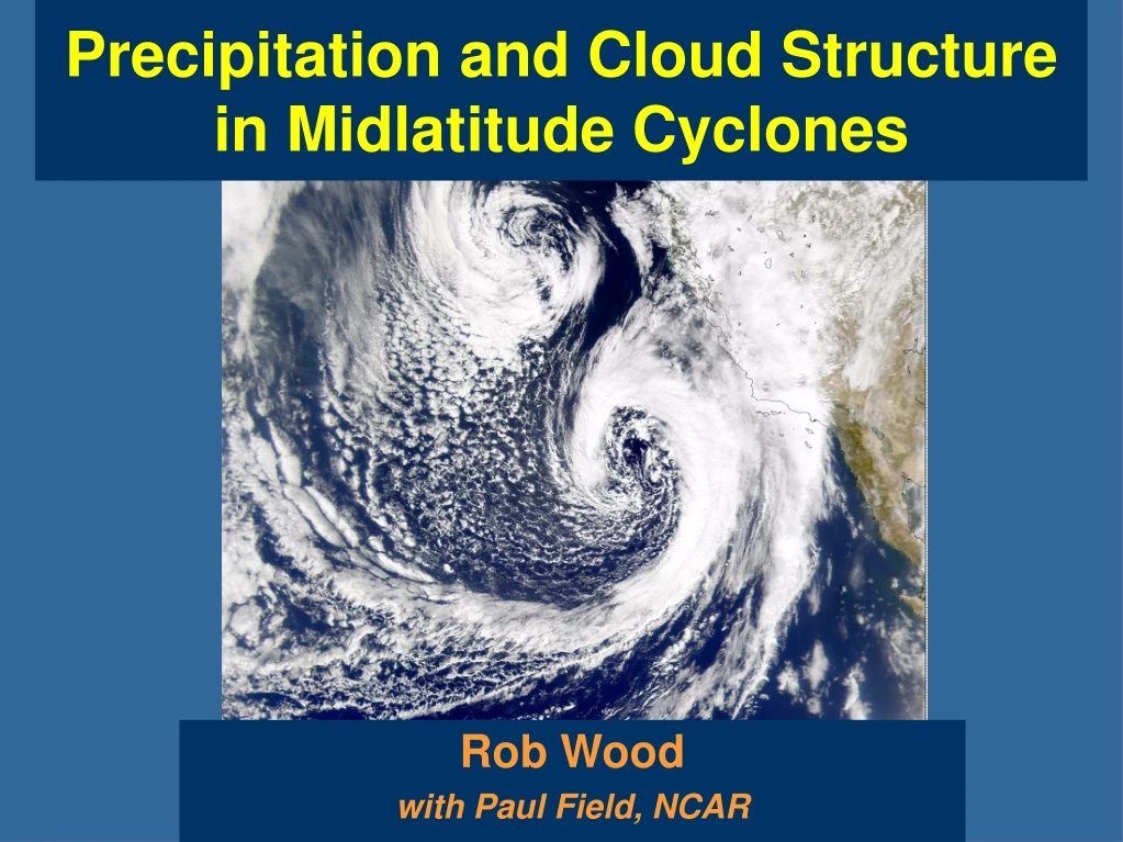
1. Precipitation and Cloud Structure in Midlatitude Cyclones Rob Wood with Paul Field, NCAR

2. stable unstable Why cyclones? Solberg (1928) examined all types of waves in the atmosphere using a two-level baroclinic model: Short waves stabilized by gravity Long waves stabilized inertially (earth’s rotation) lengthscale from Bjerknes and Holmboe, J. Met. (1944)

3. When, where? Zonal wind pressure [hPa] • Zonal winds peak in hemisphere with strongest T/y  large growth rates for baroclinic disturbances DJF Temperature 90S 60S 30S EQ 30N 60N 90N Holton, 1992

4. Hemispherical view 500 hPa geopotential height wavenumber 7   4000 km N

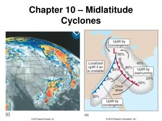
5. The structure of a midlatitude cyclone From Schultz et al. (1998) C O L D W A R M

6. Idealized cyclone Carlson 1998

7. Cyclones and climate change • Carnell and Senior (change in distribution of storm strength) • Poleward movement of the storm tracks (Fyfe, Yin, Bengtsson, Fu et al., Lorenz, Salathe…) • More precipitation/less precipitation?

8. 6 4 2 0 -2 -4 -6 -8 change in number of storms 1025 1015 1005 995 985 975 965 955 945 storm central pressure [hPa] Fewer weak storms, more strong ones? Carnell and Senior, Clim. Dyn., 1998

9. 18 15 12 9 6 3 0 Storm tracks Number of storms per month per 5x5o area Bengtsson et al. (2006)

10. Poleward storm track movement? Change in number of storms per month per 5x5o area (C 21st- C 20th) DJF JJA Also, Fu et al. (MSU), Yin, Fyfe…. 3 2 1 0 -1 -2 -3 Bengtsson et al. (2006) Mean values 5-15

11. Multisensor cyclone database • Synthesize data from useful satellite datasets and reanalysis to examine midlatitude cyclone structure • Cyclone-relative coordinate system to facilitate comparisons and composite analysis • Make available to community

12. Cloud Compositing H L Lau and Crane 1995

13. Satellite data • MODIS: Cloud top temperature and optical thickness (11o daily data) • AMSR: Rain rate; column WVP; SST • Quikscat: Surface wind speed and direction • All available data from 2003-2004 • ~2000 cyclones in total for NP, NA, SP, SA over oceanic regions • NCEP: reanalysis MSLP, T profiles (WVPsat)

14. Regions examined Major midlatitude storm track regions of the northern and southern hemispheres

15. Identifying and compositing cyclones

16. Cyclone strength and size: Region

17. Cyclone strength and size: Season Seasons reversed for SH storms

18. Quikscat winds (all NP storms) [m s-1]

19. AMSR water vapor path (all NP storms) [mm] Warm sector km

20. Warm Conveyor Belt thermodynamic dynamic R = WVPV W V S q0 = WVP / S

21. Generate new composites (combine NA, NP, SA, SP) Strength Moisture V2 r<2000 km WVP r<2000 km Quikscat windspeed WVP

23. Warm conveyor model R = WVP V • Simple model quantifies cyclone-wide precip. as a function of its strength and WVP • WVP controlled by SST Clausius -Clapeyron

24. Column mean relative humidity RHcol = WVP / WVPsat invariant to changes in storm strength or vapor

25. Cloud Top Temperature All cyclones

26. Cloud Top Temperature Normalised pdfs of composited cyclones Rainrate km km km Bjerknes and Solberg

28. Cyclones in the community atmosphere model (CAM) • Community Atmosphere Model (CAM 3.0) run for 5 years with different model configurations/parameterizations • Identical cyclone location methodology • Different model configurations: control : standard version but at 1x1o resolution micro : with new microphysics scheme (Morrison) ssat : increase critical RH for ice (from 90% to 100%) nodeep : deep convection scheme turned off noconv : deep and shallow convections schemes off 4x5 : lower resolution (4x5o)

29. Cyclone mean rain rate in CAM • Models show similar increases in R with WVP consistent with obs. • Model R is more strength-dependent than obs. models obs

30. Clausius-Clapeyron constraints • Clausius-Clapeyron constrains water vapor changes with SST in model and obs. cyclones Lapse rate changes needed to explain WVP changes z T

31. Clausius-Clapeyron constraints • Clausius-Clapeyron constrains precipitation changes in model and obs. cyclones  Large-scale precipitation changes governed by changes in cyclone strength and frequency

32. High clouds • Very sensitive to model configuration • Models show stronger moisture dependence than observations

33. Implications • dRext + dRT = LdP • LdP = k dT - 2.5 • k  3 Allen and Ingram, Nature, 2002

34. Conclusions

35. THE END

36. cloudparameterizations               Uncertainty about behavior of clouds is the leading cause of spread of temperatures under 2CO2 conditions Murphy et al. 2004 Nature Stainforth et al. 2005 Nature

37. Levels of understanding • Bjerknes – high clouds and precipitation associated with ascending regions of the cyclone • QG theory – spatiotemporal variations and strength of ascending regions understood as first order response to…. • Marriage of QG theory and moisture (latent heating) incomplete • Limitations upon what quantitative questions can be answered from a theoretical perspective (e.g. climatological response of cyclones to changing baroclinicity

38. RHwater Column (NA) km

40. But no consensus….. ECHAM-5 Bengtsson et al., J. Clim., 2006 Trends in cyclone strength dependent upon diagnostic used to define storm strength (pressure depth vs vorticity) Number per month No increase in strong storms 0 5 10 15 20 Storm intensity [10-5 s-1]

41. Compositing cyclone center