Download
1 / 66
690 likes | 866 Views
Module 3 GARCH Models. References The classics: • Engle, R.F. (1982), Autoregressive Conditional Heteroskedasticity with Estimates of the Variance of U.K, Econometrica. • Bollerslev, T.P. (1986), Generalized Autoregresive Conditional Heteroscedasticity, Journal of Econometrics.

E N D
References The classics: • Engle, R.F. (1982), Autoregressive Conditional Heteroskedasticity with Estimates of the Variance of U.K, Econometrica. • Bollerslev, T.P. (1986), Generalized Autoregresive Conditional Heteroscedasticity, Journal of Econometrics. Introduction/Reviews: • Bollerslev T., Engle R. F. and D. B. Nelson (1994), ARCH Models, Handbook of Econometrics Vol. 4. • Engle, R. F. (2001), GARCH 101: The Use of ARCH/GARCH Models in Applied Econometrics, Journal of Economic Perspectives.
• Until the early 1980s econometrics had focused almost solely on modeling the means of series -i.e., their actual values. yt = Et(yt |x) + εt , εt῀ D(0,σ2) For an AR(1) process: Et-1 (yt|x) = Et-1 (yt) = α + β yt-1 Note: E(yt) = α/(1-β)and Var(yt) = σ2/(1-β2) The conditional first moment is time varying, though the unconditional moment is not! Key distinction: Conditional vs. Unconditional moments. • Similar idea for the variance Unconditional variance: Var(yt ) = E[(yt –E[yt])2] = σ2/(1-β2) Conditional variance: Vart-1 (yt ) = Et-1[(yt –Et-1[yt])2] = Et-1[εt2]
Vart-1 (yt ) is the true measure of uncertainty at time t-1. Conditional variance variance mean
Stylized Facts of Asset Returns i) Thick tails - Mandelbrot (1963):leptokurtic (thicker than Normal) ii) Volatility clustering - Mandelbrot (1963): “large changes tend to be followed by large changes of either sign.” iii) Leverage Effects – Black (1976), Christie (1982): Tendency for changes in stock prices to be negatively correlated with changes in volatility. iv)Non-trading Effects, Weekend Effects – Fama (1965), French and Roll (1986) : When a market is closed information accumulates at a different rate to when it is open –for example, the weekend effect, where stock price volatility on Monday is not three times the volatility on Friday.
v)Expected events – Cornell (1978), Patell and Wolfson (1979), etc: Volatility is high at regular times such as news announcements or other expected events, or even at certain times of day –for example, less volatile in the early afternoon. vi) Volatility and serial correlation – LeBaron (1992): Inverse relationship between the two. vii) Co-movements in volatility – Ramchand and Susmel (1998): Volatility is positively correlated across markets/assets.
• Easy to check leptokurtosis (Stylized Fact #1) Figure: Descriptive Statistics and Distribution for EUR/ROL changes.
Changes in interest rates: Argentina, Brazil, Chile, Mexico and HK
ARCH Model - Engle(1982) Auto-Regressive Conditional Heteroskedasticity • This is an AR(q) model for squared innovations. This model cleverly estimates the unobservable (latent) variance. •Note: Since we are dealing with a variance
•Even though the errors may be serially uncorrelated they are not independent: there will be volatility clustering and fat tails. • Define standardized errors: They have conditional mean zero and a time invariant conditional variance equal to 1. That is, zt ~ D(0,1). • If, as assumed above, zt is assumed to be time invariant, with a finite fourth moment (use Jensen’s inequality): If we assume a normal distribution, the 4th moment for an ARCH(1):
More convenient, but less intuitive, presentation of the ARCH(1) model: where υt is iid with mean 0, and Var[υt]=1. Since υt is iid, the: It turns out that σt2 is a very persistent process. Such a process can be captured with an ARCH(q), where q is large. This is not efficient.
GARCH – Bollerslev (1986) In practice q is often large. A more parsimonious representation is the Generalized ARCH model or GARCH(q,p): which is an ARMA(max(p,q),p) model for the squared innovations.
This is covariance stationary if all the roots of lie outside the unit circle. For the GARCH(1,1) this amounts to • Bollerslev (1986) showed that if 3α12 + 2α1β1 + β12 < 1, the second and 4th moments of εt exist:
Forecasting and Persistence • Consider the forecast in a GARCH(1,1) model Taking expectation at time t By repeated substitutions: As j→∞, the forecast reverts to the unconditional variance: ω/(1-α1-β1). • When α1+β1=1, today’s volatility affect future forecasts forever:
Nelson’s (1991) EGARCH model Nelson, D.B. (1991), "Conditional Heteroskedasticity in Asset Returns: A New Approach," Econometrica. GJR-GARCH model Glosten, L.R., R. Jagannathan and D. Runkle (1993), "Relationship between the Expected Value and the Volatility of the Nominal Excess Return on Stocks," Journal of Finance. where It-i=1 if εt-i<0; 0 otherwise. • Both models capture sign (asymmetric) effects in volatility:Negative news increase the conditional volatility (leverage effect).
Non-linear ARCH model NARCH Higgins and Bera (1992) and Hentschel (1995) These models apply the Box-Cox transformation to the conditional variance. Special case: γ=2 (standard GARCH model). • The variance depends on both the size and the sign of the variance which helps to capture leverage type (asymmetric) effects.
Threshold ARCH (TARCH) Rabemananjara, R. and J.M. Zakoian (1993), “Threshold ARCH Models and Asymmetries in Volatilities,”Journal of Applied Econometrics. Large events to have an effect but no effect from small events There are two variances: Many other versions are possible by adding minor asymmetries or non-linearities in a variety of ways.
Switching ARCH (SWARCH)Hamilton, J. D. and R. Susmel (1994), "Autoregressive Conditional Heteroskedasticity and Changes in Regime," Journal of Econometrics. • • Intuition: • - Hamilton (1989) models time series with changes of regime. • Simplest case: 2-state process. • - Hamilton assumes the existence of an unobserved variable, st, that can take two values: one or two (or zero or one). • - Hamilton postulates a Markov transition matrix, P, for the evolution of the unobserved variable: • p(st =1 | st-1 =1) = p • p(st =2 | st-1 =1) = (1-p) • p(st =1 | st-1 =2) = q • p(st =2 | st-1 = 2) = (1-q)
Reformulate ARCH(q) equation to make the conditional variance dependent on st –i.e., the state of the economy. • • A parsimonious formulation: For a SWARCH(1) with 2 states (1 and 2) we have 4 possible σt2:
• The parameter γst=1 is set to 1. Then, the parameter γst=2 is a relative volatility scale parameter. If γst=2 =3, then volatility in the state 2 is three times higher than in state 1. • In SWARCH models, the states refer to the states of volatility. For a 2-state example, we have “high,” or “low” volatility states. Since we have an unobservable variable, estimation is usually done with a variation of the Kalman filter model. • Estimation of the model will estimate the volatility parameters, and the transition probabilities. As a byproduct of the estimation, we will also have an estimate for the latent variable –i.e., the “state.”
Integrated GARCH (IGARCH) The standard GARCH model is covariance stationary if • But strict stationarity does not require such a stringent restriction (That is, that the unconditional variance does not depend on t). If we allow α1 + β1 =1, we have the IGARCH model. • In the IGARCH model the autoregressive polynomial in the ARMA representation has a unit root: a shock to the conditional variance is “persistent.”
Today’s variance remains important for future forecasts of all horizons. • This is the Integrated GARCH model (IGARCH). • Nelson (1990) establishes that, as this satisfies the requirement for strict stationarity, it is a well defined model. • In practice, it is often found that α1 + β1 are close to 1. • We may suspect that IGARCH is more a product of omitted structural breaks than the result of true IGARCH behavior. See Lamoreux and Lastrapes (1989) and Hamilton and Susmel (1994).
FIGARCH ModelBaillie, Bollerslev and Mikkelsen (1996), Journal of Econometrics. • Recall the ARIMA(p,d,q) model (1-L)d α(Lp)yt=β(Lq)εt, where εt, is white noise.When d=1, we have yt is an Integrated process. In time series, it is usually assumed that d=1,2,…D.• But it can be any positive number, for example, 0<d<1. In this case, we have a fractionally integrated process, or ARFIMA. (See Granger and Joyeaux (1980).)•d is called the fractional integration parameter. • When d €{-1/2,1/2}, the series is stationary and invertible. Hoskings (1981).
• Similar intuition carries to the GARCH(q,p) model. • Recall the ARMA representation for GARCH process: • Now, the FIGARCH process is defined as: • When d=0, we have a GARCH(q,p), when d=1, we have IGARCH. • This model captures long-run persistent (memory).
• Questions1) Lots of ARCH models. Which one to use?2) Choice of p and q. How many lags to use? • • Hansen and Lunde (2004) compared lots of ARCH models: • - It turns out that the GARCH(1,1) is a great starting model. • - Add a leverage effect for financial series and it’s even better.
Estimation: MLE All of these models can be estimated by maximum likelihood. First we need to construct the sample likelihood. Since we are dealing with dependent variables, we use the conditioning trick to get the joint distribution: Taking logs
Assuming normality, we maximize with respect to θ the function: Example: ARCH(1) model. Taking derivatives with respect to θ=(ω,α,γ), where γ=K mean pars:
Note that the δϑ/δγ=0 (K f.o.c.’s) will give us GLS.Denote δϑ/δθ=S(yt,θ)=0 (S(.) is the score vector) • We have a (K+2xK+2) system. But, it is a non-linear system. We will • need to use numerical optimization. • • Gauss-Newton or BHHH can be easily implemented. • • Given the AR structure, we will need to make assumptions about σ0 • (and ε0,ε1 , ..εp if we assume an AR(p) process for the mean). • Alternatively, we can take σ0 (and ε0,ε1 , ..εp) as parameters to be • estimated (it can be computationally more intensive and estimation • can lose power.)
Note: The appeal of MLE is the optimal properties of the resulting estimators under ideal conditions.Crowder (1976) gives one set of sufficient regularity conditions for the MLE in models with dependent observations to be consistent and asymptotically normally distributed. Verifying these regularity conditions is very difficult for general ARCH models - proof for special cases like GARCH(1,1) exists. For GARCH(1,1) model: if E(ln α1,zt2 +β1] < 0, the model is strictly stationary and ergodic. See Lumsdaine (1992).
If the conditional density is well specified and θ0 belongs to Ω, then • • Common practice in empirical studies: Assume the necessary regularity conditions are satisfied. • Under the correct specification assumption, A0=B0, where We estimate A0 and B0 by replacing θ0 by its estimated MLE value. The estimator B0 has a computational advantage over A0.: Only first derivatives are needed. But A0=B0 only if the distribution is correctly specified. This is very difficult to know in practice.
• Block-diagonality In many applications of ARCH, the parameters can be partitioned into mean parameters, θ1, and variance parameters, θ2. Then, δμt(θ)/δθ2=0 and, although, δσt(θ)/δθ1≠0, the Information matrix is block-diagonal (under general symmetric distributions for zt and for particular ARCH specifications). Not a bad result: - Regression can be consistently done with OLS. - Asymptotically efficient estimates for the ARCH parameters can be obtained on the basis of the OLS residuals. • But block diagonality can’t buy everything: - Conventional OLS standard errors could be terrible. - When testing for serial correlation, in the presence of ARCH, the conventional Bartlett s.e. – (1/n)-1- could seriously underestimate the true s.e.
Estimation: QMLE • The assumption of conditional normality is difficult to justify in many empirical applications. But, it is convenient. • The MLE based on the normal density may be given a quasi-maximum likelihood (QMLE) interpretation. • If the conditional mean and variance functions are correctly specified, the normal quasi-score evaluated at θ0 has a martingale difference property: E{δϑ/δθ=S(yt,θ0)}=0 Since this equation holds for any value of the true parameters, the QMLE, say θQMLE is Fisher-consistent –i.e., E[S(yT, yT-1,…y1 ; θ)] = 0 for any θ€Ω.
• The asymptotic distribution for the QMLE takes the form: The covariance matrix (A0-1 B0 A0-1) is called “robust.” Robust to departures from “normality.” • Bollerslev and Wooldridge (1992) study the finite sample distribution of the QMLE and the Wald statistics based on the robust covariance matrix estimator: For symmetric departures from conditional normality, the QMLE is generally close to the exact MLE. For non-symmetric conditional distributions both the asymptotic and the finite sample loss in efficiency may be large.
Estimation: GMM • Suppose we have an ARCH(q). We need moment conditions: Note: (1) refers to the conditional mean, (2) refers to the conditional variance, and (3) to the unconditional mean. GMM objective function: where
• γ has K free parameters; α has q free parameters. Then, we have a=K+q+1 parameters. • m(θ;X,y) has r=k+m+2 equations. • Dimensions: Q is 1x1; E[m(θ;X,y)] is rx1; W is rxr. • Problem is over-identified: more equations than parameters so cannot solve E[m(θ;X,y)]=0, exactly. • Choose a weighting matrix W for objective function and minimize using nonlinear solver (for example, optmum in GAUSS). • Optimal weighting matrix: W =[E[m(θ;X,y)]E[m(θ;X,y)]’]-1. • Var(θ)=(1/T)[DW-1D’]-1, where D = δE[m(θ;X,y)]/δθ’. (all these expressions evaluated at θ^.)
TestingWhite’s (1980) general test for heteroskedasticity.Engle’s (1982) TR2~χ2q • • In ARCH Models, testing as usual: LR, Wald, and LM tests. • Reliable inference from the LM, Wald and LR test statistics • generally does require moderately large sample sizes of at least two • hundred or more observations. • • Issues: • - Non-negative constraints must be imposed. θ0 is often on the • boundary of Ω. (Two sided tests may be conservative) • - Lack of identification of certain parameters under H0, creating a • singularity of the Information matrix under H0. For example, under • H0:α1=0 (No ARCH), in the GARCH(1,1), ω and β1 are not jointly • identified. See Davies (1977).
Ignoring ARCH Hamilton, J.D. (2008), “Macroeconomics and ARCH, Working paper, UCSD. • Many macroeconomic and financial time series have an AR structure. What happens when ARCH effects are ignored? Assume yt = γ0 + γ1 yt-1 + εt , where εt follows a GARCH(1,1) model. Then, ignoring ARCH: Assume the 4th moment exists, standard consistency give us
For simplicity assume γ0=0. Then, T1/2γ is approximately N(0,1). But, Under H0: No ARCH, the second summation is a MDS with variance Using CLT: To calculate the value of the variance, recall the ARMA(1,1) representation for GARCH(1,1) models:
For an ARMA(1,1): Then, after some substitutions: Note: V11 ≥1, with equality iff α1=0. OLS treats T1/2γ^ as N(0,1), but the true asymptotic distribution is N(0,V11). OLS tests reject more often. As α1 and β1 get closer to μ4=∞, we reject even more.
Figure 1. (From Hamilton (2008).) Asymptotic rejection probability for OLS t-test that autoregressive coefficient is zero as a function of GARCH(1,1) parameters α and δ. Note: null hypothesis is actually true and test has nominal size of 5%.
• If the ARCH parameters are in the usual range found in estimates of GARCH models, an OLS t-test with no correction for heteroskedasticity would spuriously reject with arbitrarily high probability for a sufficiently large sample. • • The good news is that the rate of divergence is slow: • it may take a lot of observations before the accumulated excess • kurtosis overwhelms the other factors. • The solid line in Figure 2 plots the fraction of samples for which an • OLS t test of γ1= 0 exceeds two in absolute value. Thinking we’re • only rejecting a true null hypothesis 5% of the time, we would do so • 15% of the time when T = 100 and 33% of the time when T = 1,000. • • White’s (1980) s.e. help. Newey-West’s (1987) s.e. help less. • • Engle’s TR2 is very good. Better than White’s (1980), as expected
Figure 2. From Hamilton (2008). Fraction of samples in which OLS t-test leads to rejection of the null hypothesis that autoregressive coefficient is zero as a function of the sample size for regression with Gaussian errors (solid line) and Student’s t errors (dashed line). Note: null hypothesis is actually true and test has nominal size of 5%.
ARCH in MEAN (G)ARCH-M Engle, R.F., D. Lilien and R. Robins (1987), “Estimating Time Varying Risk Premia in the Term Structure: the ARCH-M Model,” Econometrica. • Finance theory suggests that the mean of a relationship will be affected by the volatility or uncertainty of a series. ARCH in mean (ARCH-M) framework: The variance or the standard deviation are included in the mean relationship.
The difference from the previous models ARCH/GARCH models is that the volatility enters also in the mean of the return. • This is exactly what Merton’s (1973, 1980) ICAPM produces • risk-return tradeoff. It must be the case that δ> 0. • Again, we have a Davies (1977)-type problem. Let μt(θ)= μ +δσt(θ), with μ≠0 , δis only identified if the conditional variance is time-varying. Thus, a standard joint test for ARCH effects and δ= 0 is not feasible. Note: Block-diagonality does not hold for the ARCH-M model. Consistent estimation requires correct specification of cond. mean and variance. (And simultaneous estimation.)
Non normality assumptions The basic GARCH model allows a certain amount of leptokurtosis. It is often insufficient to explain real world data. Solution: Assume a distribution other than the normal which help to allow for the fat tails in the distribution. • t Distribution - Bollerslev (1987) The t distribution has a degrees of freedom parameter which allows greater kurtosis. The t likelihood function is where Γis the gamma function and v is the degrees of freedom. As υ→∞, this tends to the normal distribution. • GED Distribution - Nelson (1991)
Multivariate ARCH ModelsEngle, R.F. and K.F. Kroner (1993), Multivariate Simultaneous Generalized ARCH, working paper, Department of Economics, UCSD. • It is common in Finance to stress the importance of covariance • terms. The above model can handle this if y is a vector and we • interpret the variance term as a complete covariance matrix. The • whole analysis carries over into a system framework: • From an econometric theory point of view, multivariate ARCH models add no problems. The log likelihood assuming normality is:
• Several practical issues: -A direct extension of the GARCH model would involve a very large number of parameters (for 4 assets, we have to estimate 10 elements in Ωt). -The conditional variance could easily become negative even when all the parameters are positive. -The chosen parameterization should allow causality between variances. - Covariances and Correlations: How to model them?
Vector ARCH Let vech denote the matrix stacking operation A general extension of the GARCH model would then be W is vector with T(T+1)/2 elements, A(L) and B(L) are squared matrices with T(T+1)/2xT(T+1)/2 elements. Total parameters: T(T+1)/2 +T2 (T+1)2/2. This quickly produces huge numbers of parameters, for p=q=1 and n=5 there are 465 parameters to estimate here.