Approximability of Combinatorial Optimization Problems with Submodular Cost Functions
520 likes | 754 Views
Approximability of Combinatorial Optimization Problems with Submodular Cost Functions. Pushkar Tripathi Georgia Institute of Technology. Based on joint work with Gagan Goel , Chinmay Karande , and Wang Lei. Motivation . Network Design Problem. f. g. h.

Approximability of Combinatorial Optimization Problems with Submodular Cost Functions
E N D
Presentation Transcript
Approximability of Combinatorial Optimization Problems with Submodular Cost Functions PushkarTripathi Georgia Institute of Technology Based on joint work with GaganGoel, ChinmayKarande, and Wang Lei
Motivation Network Design Problem f g h Objective: Find minimum spanning tree that can be built collaboratively by these agents
Functions which capture economies of scale Additive Cost Function cost(a) = 1 cost(b) = 1 cost(a,b) = 2 cost(a) = 1 cost(b) = 1 cost(a,b) = 1.5 How to mathematically model these functions? - We use Submodular Functions as a starting point. Can one design efficient approximation algorithms under Submodular Cost Functions?
Assumptions over cost functions • Normalized: • Monotone: • Decreasing Marginal: Submodularity + + ≥ Submodular Functions
General Framework • Ground set X and collection C µ2X • C: set of all tours, set of all spanning trees • k agents, each specifies fi: 2X→ R+ • fi issubmodular and monotone • Find S1, …, Sk such that: • [Si2 C • ifi(Si) is minimized S ORACLE f(S)
Our Results Lower Bounds : Information theoretic Upper Bounds : Rounding of configurational LPs, Approximating sumdodular functions and Greedy Single Agent Multiple Agents
Selected Related Work • [Grötschel, Lovász, Schrijver 81] Minimizing non-monotone submodular function is poly-time • [Feige, Mirrokni, Vondrak 07] Maximizing non-monotone function is hard. 2/5-Approximation Algorithm. • [Calinescu, Chekuri, Pal, Vondrak 08] Maximizing monotone function subject to Matroid constraint: 1-1/e Approximation. • [Svitkina, Fleischer 09] Upper and lower bounds forSubmodular load balancing, Sparsest Cut, Balanced Cut • [Iwata, Nagano 09] Bounds for Submodular Vertex Cover, Set Cover • [Chekuri, Ene 10] Bounds for SubmodularMultiway Partition
In this talk • Submodular Shortest Path with single agent • O(n 2/3) approximation algorithm • Matching hardness of approximation
In this talk • Submodular Shortest Path with single agent • O(n 2/3) approximation algorithm • Matching hardness of approximation
Submodular Shortest Path t s G=(V,E) |V| =n , |E| =m Given: Graph G, Two nodes s and t f : 2E→ R+ Submodular, Monotone Goal: Find path P s.t. f(P) is minimized
Attempt 1: Approximate by Additive function • Let we = f({e}) • Idea : we· OPT · we e 2 OPT e 2 OPT t • 1. Guess • e* = argmax{we| e 2OPT } s • 2. Pruning: Remove edges costlier than e* • 3. Search: Find the shortest length s-t path in the residual graph ALG · diameter(G’).we*· diameter(G’).OPT
Attempt 2: Ellipsoid Approximation John’s theorem : For every polytope P, there exists an ellipsoid contained in it that can be scaled by a factor of O(√n) to contain P P [GHIM 09]: If the convex body is a polymatroid, then there is a poly-time algorithm to compute the ellipse.
Attempt 2: Ellipsoid Approximation P [GHIM 09]: If the convex body is a polymatroid, then there is a poly-time algorithm to compute the ellipse. ∀S: ∑e 2 S x(e) ≤ f(S) ∀e: x(e) ≥ 0 f: Submodular, monotone Polymatroid
Approximating Submodular Functions Polynomial time d4 d5 f : Monotone submodular function d1 d6 |X| = n d3 d2 g(S) = √ de e 2 S X g(S) · f(S) ·√ n g(S)
Attempt 2: Ellipsoid Approximation STEP 1: [GHIM ‘09] f: 2E→ R+ Submodular, Monotone g(S): = √ de {de} STEP 2: Min g(S) s.t. S 2 PATH(s,t) * Minimizing over g(S) is equivalent to minimizing just the additive part Analysis: f(P) ≤ g(P) ≤ g(O) ≤ f(O) P: Optimum path under g O: Optimum path under f √E √E √E
Recap. • Approximating by linear functions : Works for graphs with small diameter • Approximating by ellipsoid functions : Works for sparse graphs n/2 n/2 Dense Graph with large diameter
Algorithm for Shortest Path STEP 1: Pruning - Guess edge e* = argmax {we | e ϵ OPT path} - Remove edges costlier than we*
Algorithm for Shortest Path STEP 1: Pruning - Guess edge e* = argmax {we | e ϵ OPT path} - Remove edges costlier than we* STEP 2 : Contraction -if ∃ v , s.t. degree(v) > n1/3, contract neighborhood of v - repeat
s s t t Dense connected component
Algorithm for Shortest Path STEP 1: Pruning - Let we = f({e}) - Guess edge e* = argmax {we | e ϵ OPT path} - Remove edges costlier than we* STEP 2 : Contraction -if ∃ v , s.t. degree(v) < n1/3, contract neighborhood of v - repeat STEP 3 : Ellipsoid Approximation -Calculate ellipsoidal approximation (d,g) for the residual graph
Algorithm for Shortest Path STEP 1: Pruning - Let we = f({e}) - Guess edge e* = argmax {we | e ϵ OPT path} - Remove edges costlier than we* STEP 2 : Contraction -if ∃ v , s.t. degree(v) < n1/3, contract neighborhood of v - repeat STEP 3 : Ellipsoid Approximation -Calculate ellipsoidal approximation (d,g) for the residual graph STEP 4 : Search -Find shortest s-t path according to g.
s t
Algorithm for Shortest Path STEP 1: Pruning - Let we = f({e}) - Guess edge e* = argmax {we | e ϵ OPT path} - Remove edges costlier than we* STEP 2 : Contraction -if ∃ v , s.t. degree(v) < n1/3, contract neighborhood of v - repeat STEP 3 : Ellipsoid Approximation -Calculate ellipsoidal approximation (d,g) for the residual graph STEP 4 : Search -Find shortest s-t path according to g. STEP 5 : Reconstruction -Replace the path through each contracted vertex with one having the fewest edges.
Path having fewest edges s t
Analysis s R P1 P2 t
Bounding the cost of P1 P1 P2 s R f(P1) ≤ √ E(R) .g(P1) ≤ √ E(R).g(OPT) ≤ √ E(R) .f(OPT) ≤ n2/3 f(OPT) Has at most n4/3 edges t
Bounding the cost of P2 G1 Diam(Gi) · |Gi|/n1/3 s G2 f(P2) ≤ (dia(G1) +.. +dia(Gk) ) we* ≤ (|G1| / n1/3 + …. ) we* ≤ (n / n1/3) we* ≤ n2/3 f(OPT) G3 t
In this talk • Submodular Shortest Path with single agent • O(n 2/3) approximation algorithm • Matching hardness of approximation
Information Theoretic Lower Bound • Polynomial number of queries to the oracle • Algorithm is allowed unbounded amount of time to process the results of the queries • Not contingent on P vs NP f(S1) S1 f(S2) S2 f f(S2) S3
General Technique • Cost functions f , g satisfying • OPT( f ) >> OPT( g ) • f (S) = g(S)for ‘most’ sets S • A – any randomized algorithm • f(Q ) = g( Q )with high probability for every query Q made by A. Probability over random bits in A.
Yao’s Lemma f(Q) = g(Q) with high probability for every query Q made by randomized algorithm A. fand a distribution D from which we choose g, such that for an arbitrary query Q , f(Q) = g(Q) with high probability
Non-combinatorial Setting X : Ground set f(S) = min{ |S|, ® } D : R µ X, |R| = ® gR(S) = min{| S ÅRc| +min( S Å R, ¯ ) }
Optimal Query Claim : Optimal query has size ® Case 1 : |Q| < ® Probability can only increase if we increase |Q|
Case 2 : |Q| > ® Probability can only increase if we decrease |Q| Optimal query size to distinguish f and gR is ®
Distinguishing f and gR Chernoff Bounds ¯ = (1+ ±) E[|Q Å R|] f and g are hard to distinguish
Hardness of learning submodular functions • Set ® = n1/2log n • Optimal query size = ® = n1/2log n • |R| = ® = n1/2log n • E[ Q Å R] = log2n • ¯ = (1+±) E[ Q Å R] = (1+±)log2n Super logarithmic f and g are indistinguishable f(R) = min{ |R|, ® } = |R| = ® = n1/2 log n gR(R) = min{| R ÅRc| +min( R Å R, ¯ ) } = ¯ = log2 n Corollary : Hard to learn a submodular function to a factor better than n1/2/log n in polynomial value queries.
Difficulty in Combinatorial Setting • Randomly chosen set may not be a feasible solution in the combinatorial setting. Eg. Randomly chosen set of edges rarely yield a s-t path. Solution : Do not choose R randomly from the entire domain X. Use a subset of R as a proxy for the solution.
Base Graph G s …... t n1/3 vertices n2/3 levels
Functions f and g Y ……. ……. s t B f(S) = f( S Å B ) & g(S) = g( S Å B )
Functions f and g Y ……. ……. s t B f(S) = min( |S Å B|, α)
Functions f and g Solution : Do not choose R randomly from the entire domain X. Use a subset of R as a proxy for the solution. Y ……. ……. s t Uniform random subset of B of size ® B gR(S) = min{| S Å R Å B| +min( S Å R Å B, ¯ )}
Functions f and g Solution : Do not choose R randomly from the entire domain X. Use a subset of R as a proxy for the solution. Y R = n2/3log2 n ……. ……. s t B gR(S) = min{| S Å R Å B| +min( S Å R Å B, ¯ )
Setting the constants • Set ® = n2/3log2 n • Optimal Query size = ® = n2/3log2 n • ¯ = log2 n f and g are indistinguishable f(OPT) = min{ |R|, ® } = |R| = ® = O(n2/3log2 n) gR(OPT) = min{| R ÅRc| +min( R Å R, ¯ ) } = ¯ = log2 n Theorem : Submodular Shortest Path problem is hard to approximate to a factor better than O(n2/3)
Summary Single Agent Multiple Agents n: # of vertices in graph G What’s the right model to study economies of scale?
Newer Models • Discount Models f E R E R E R g h
Task: Minimize sum of payments Payment Sub modular functions Cost f(a) + f(b) + f(c) ….
Approximability under Discounted Costs[GTW 09] O(log n) O(log n) O(poly log n)
Shortest Path : O(logc n) hardness s S U t Agents - Cost of every edge is 1 1 1 Set Cover Instance Claim : Set cover of size |S| ↔ Shortest path of length |S|
Hardness Gap Amplification s s t Original Instance • Replace each edge by a copy of the original graph. • Edges of the same color get the same copy. • Edges of different colors gets copies with new colors(agents) t Harder Instance
Claim : The new instance has a solution of cost α2iff the original instance has a solution of cost α. • For any fixed constant c iterate this construction c times to further amplify the lower bound to O(logcn).