Download
1 / 37
370 likes | 431 Views
Optimizing Economic Return in egg production. Steve Wilcox Senior Mathematics Major Northern Kentucky University April 29, 2011. The Story. A Shaver White Chicken.

E N D
Optimizing Economic Return in egg production Steve Wilcox Senior Mathematics Major Northern Kentucky University April 29, 2011
The Story A Shaver White Chicken Randy Weibe currently keeps his Shaver White Chickens for about 51 weeks at a time. The chickens are obtained at 19 weeks of age and the hen producers recommends that hens be “disposed of” at 70 weeks -- hence the 51 weeks. We suspect that they are productive beyond 70 weeks. How can we prove this?
The Data Randy noting the number of eggs for the day. • Extra Large Eggs • Large Eggs • Medium Eggs • Small Eggs • PeeWee Eggs • Grade B • Grade C / Cracked • Rejects • Randy collects data over an entire cycle of egg production. • Total eggs produced each day • “Gradeout” information: breakdown of the size and quality of the eggs received in Winnipeg.
The Egg Production Cycle • We used Randy’s data to estimate the average daily profit from his eggs during the egg production phase. As long as the average is high, we will keep these hens in production. • An egg production cycle is in two parts: the production phase, when the chickens are laying eggs, and the very expensive transition phase when chickens are being replaced, barns are being cleaned, etc. Costs of the transition phase are well understood.
The Average Daily Return • Cost for daily operations (hen maintenance) • Cost of downtime (time in-between old and new hens) • Price of the eggs • Daily egg production • Gradeouts from the egg buyers • We want to maximize the average daily return over a complete cycle. • To do this, we created a model consistent with the following five factors:
Finding a Model – Economics • One of the things we consider is the economics of the process. • The economics of the process consists of the return the farmer is gaining from selling eggs versus the costs required to purchase, maintain, and dispose of the chickens. (“Profit=money in - money out.) • The farmer is gaining money from the eggs, but losing money based on several factors.
Model – Economics • On the negative side, the farmer is paying for the cost of maintenance on the chickens. • e.g. feed for the chickens and cleaning supplies to keep the facility sanitary. • Another negative input to the economics is the “downtime”. • This is the time interval in which old hens are disposed of, new hens are being purchased, and no eggs are being produced.
Model – Economics • On the positive side, the farmer is gaining money from the eggs being produced. • For our purposes, the amount of money for each type of egg (grade) was set to a fixed price, the most common prices for this cycle. • The information provided to us is daily production numbers and the gradeouts the farmer receives weekly.
Model – Gradeouts • The different gradeout types and set prices are as follows: • Extra Large Eggs - $1.54 / dozen • Large Eggs - $1.54 / dozen • Medium Eggs - $1.36 / dozen • Small Eggs - $0.94 / dozen • Peewee Eggs - $0.2425 / dozen • Grade “B” Eggs - $0.45 / dozen • Grade C Eggs (Cracked) - $0.15 / dozen • Rejected Eggs - $0.00 / dozen
Model – Gradeouts • The “gradeouts” are essentially the invoices which lists how many eggs of each type were produced. • It also lists the current price for each grade and how much gross income was made off of each grade type. • Again, for simplicity, we are setting the price for each egg grade to a constant.
Modeling Daily Egg Revenue If we look at the graph of the daily egg revenue over time (with all gradeouts combined), we see three phases: an increasing phase, a short stable plateau, and a decreasing phase.
The Model 1 P(t) = -c*t 1+e Our data suggests incorporating some “S-curves” (e.g. “logistic” models) to handle these three phases. A typical logistic function:
The Model - Daily Egg Gross Return R(t)= • Where: • c is the height parameter of the first logistic. • a1 is the central steepness of the first logistic. • a2 is the central steepness of the second logistic. • b1 is the center location for the first logistic. • b2 is the center location for the second logistic. • We decided on a model which consists of the product of two logistic functions. • One is increasing (production ramping up) and the other is a decaying logistic (hens winding down). • Our Daily Return Model during production:
Using the Model • Now that we have the model, it is possible for us to calculate the total area underneath the logistic curve. This will give us the total number of eggs produced over the course of the chicken’s lives. • However, this is not what we were interested in. Even though it does help us get to where we want to go, we still have a few more things to get what we are looking for: the total economic value of these eggs.
Using the Gradeout Data The gradeouts provide us data that tells us the percentage and total number of eggs (in dozens) produced in a particular week. From this, we can calculate an economic value for this particular week, based on these percentages given to us and the cost for each type of egg.
Using the Gradeouts Note: On this particular day, 11,700 dozen eggs were produced in total. Egg Type Percentage Total (dozens) Egg Type Percentage Total (dozens) • Extra Large 14.56% 1704 • Large 57.15% 6687 • Medium 24.12% 2822 • Small 0.65% 76 • Peewee 0.00% 0 • B 0.36% 42 • Cracked 1.82% 213 • Rejects 1.33% 156 • We then multiply the total number of eggs by the value of the egg types ($1.54 for the extra large eggs and the large eggs, $1.36 for the medium eggs, etc). This gives us the total economic value for that week’s worth of egg production. • The problem with this is that we need daily gradeouts, not just weekly gradeouts. This way we can assign a particular economic value to each day instead of each week. How could we possibly achieve this? For example, the 46th week had the following data:
Interpolation In order to obtain the daily values, we need to use interpolation on the data. Interpolation is when you estimate intermediate data values based on known data points. In our case, we know the grades from week to week. By using interpolation, we are able to estimate daily gradeouts based on adjacent weeks of data.
Interpolation Proportion of Large Eggs .63 .59 Week 25 Week 24 We chose a conservative method: linear splines, a standard type of interpolation (effectively we are just “connecting the dots” to estimate between).
Calculating the Economic Value From here, we can now integrate the model over a span of time in order to estimate the total return that Randy can expect from one egg production cycle. After we obtain the total value of the eggs, we must then subtract all fees for maintenance during production, and the costs of the transition period, such as the daily living cost of the chickens (e.g. chicken feed), the cost for disposal of the chickens, the cost of cleaning the barns, etc.
Economic Model – Average Daily Return ADR(D)= D = duration of the egg production phase. CPD = Cost per Day during egg production (Randy provided $1,712.91). TTC = Total Transition Cost (Randy provided $139,091.20). TTT = Total Transition Time (Randy provided 10 days).
Looking at the graph of the Economic Function This is what the product of two logistics looks like. The downtime (in red) corresponds to TTT in the formula, it is the amount of time for the transition from old chickens to new ones (in days) The green region indicates the total value of the egg production over the duration (then all the daily costs are taken out).
Problems If you remember back to the beginning, we said that chickens must be raised to the age of 19 weeks before they even start producing eggs. But what does this mean for our model?
Problems This means that we must be able to predict at least 19weeks in advance when the appropriate time is to call for the next batch of hens.
Problems • If we have a good model, we should have well enough time to predict when the cut-off time period should be. • This cut-off period should include a “grace” period in which Randy will actually be able to make preparations for new chickens. He wouldn’t reasonably be able to expect new chickens to be started the very next day.
Calculating the best cut-off day • To optimize the number of days to keep the chickens in production, we take the derivative of the economic model and then set this equal to 0. • With this data, we would be able to calculate the amount of money he would have made on a daily basis based on the day the chickens were kept alive and producing. We can then use these to compare how much of a difference keeping the chickens longer will affect Randy’s profits.
Back-Tracking to calculate the day “D” in our economic model Backing up and using the model at day 171 gives us the following graph: This tells us that the chickens have not even started to drop in number of eggs produced. Using our data, we back-tracked to determine if this model was able to accurately predict a good “cut-off” time 19 weeks in advance. At this point, only the first logistics function is affect the data.
Back-Tracking At this point, the egg production has started to drop (and the second logistic function can be seen). At this point, Randy should be watching his data to see when the economic value of the eggs will drop as well. Here is what the data looks like if we start at day 240.
Back-Tracking If we do this enough, we can look at the projected time for the optimal duration that the flock should be kept to obtain maximum economic value. At around day 280, we can see that it appear the data seems to be converging to a particular “optimal” day, in this case the data appears to be converging to around day 436. If we were to keep the chickens to day 436, as the graph appears to be saying thus far, then at day 280, we still have 22 weeks before the old chickens will need to be replaced. If Randy starts making preparations at this point, he will have about 3 weeks to make preparations for the new batch of chickens.
The Results We want to take the derivative of this function to find the maximum So it looks like from this graph that the maximum economic value of these chickens peaks at around day 436 or so (which is a little over 62 weeks) • This is what the Average Daily Return looks like:
The Results After taking a derivative and setting the function equal to 0, then solving, we get the following data points: • If he did keep the chickens for 357 days (as the manufacture suggested) then Randy would have made a maximum of $275.87 dollars a day. • By keeping them for 371 days, Randy only made a maximum of $285.18 dollars a day. • If he would have kept them for 436 days instead, Randy would have made up to $303.76 dollars a day. This is about 18 dollars a day more than what he actually made. Over the course of a year, that adds up to about $6500.00 more he could have made.
The Results So, according to the model that we have found, we predict that Randy’s chickens could have lived up to 62 weeks after the began ovulation, or to around week 81 of their lives. What does this mean? These chickens never got the chance to reach their maximum economic value! They were killed 11 weeks prior to this time period.
Should we believe the model? • Assuming the trend is believable, we can say that it would be beneficial to Randy to keep the chickens for 11 weeks longer. • However, this model • assumes a consistent trend • after our last set of data • points. We have no way to • know for sure that these • chickens would continue • producing as before. That is, • we have no way to know • whether or not the chickens • would just suddenly stop • producing after day 371.
Should we believe the model? • This shows us that these chickens are capable of producing eggs long after the age of 81 weeks, even up to 100 or 105 weeks. • So yes, I believe the model is believable. Here is a picture of an example of Shaver White Chicken data with more than 71 weeks of egg production.
Future Works Naturally, the model isn’t perfect and it’s possible that we did not look at this model from as many angles as we could have to capture the whole picture. The following slides consists of suggestions I have that may help improve this model in the future.
Fine Tuning the model – Mortality • Perhaps another factor we could have included to the model is the mortality of the chickens. • Naturally, as time goes on and chickens get older, exhausted, or otherwise worn down; some of the chickens will start to die off. • This has another negative impact on the economic value of the current chickens that are in house.
Fine Tuning the model – Mortality • Mortality Effect: • Even if chickens are producing eggs as well as ever, a smaller number of chickens still means a smaller number of eggs. • This, of course, means less gradeouts; which in turn is hurting the economic value of the current chickens.
Acknowledgments • Thanks to Randy Weibe for providing the data and answers to several chicken-related questions. • Thanks to Dr. Long for his willingness to help me with this capstone and all the help he provided along the way. • http://www.hotelmule.com/attachments/2009/08/26_20090824062802439gB.gif • Picture for egg sizes • http://www.worldpoultry.net/public/image/ISA%20graph.JPG • Picture for egg production after 52 weeks.