Particle System
Computer Animation Lecture 12. Particle System. Particle Systems For Nature Effects. The use of Particle systems is a way of modelling fuzzy objects, such as fire, clouds, smoke, water, etc. These objects don't have smooth well-defined surfaces and are non-rigid

Particle System
E N D
Presentation Transcript
Computer Animation Lecture 12 Particle System
Particle Systems For Nature Effects • The use of Particle systems is a way of modelling fuzzy objects, such as • fire, • clouds, • smoke, • water, etc. • These objects don't have smooth well-defined surfaces and are non-rigid • Use small particles to represent them
Advantages of using Particle Systems Complex systems can be created with little human effort. The level of detail can be easily adjusted. For example, if a particle system object is in the distance, then it can be modelled to low detail (few particles), but if it is close to the camera, then it can be modelled in high detail (many particles)
Basic Model of Particle Systems A particle system is a collection of many minute particles that model some object. For each frame of an animation sequence the following steps are performed: • New particles are generated • Each new particle is assigned its own set of attributes • Any particles that have existed for a predetermined time are destroyed • The remaining particles are transformed and moved according to their dynamic attributes • An image of the remaining particles is rendered
Particle Generation • Particles are generated using stochastic methods. • the designer controls the mean number of particles generated per frame and the variance. • So the number of particles generated at frame F is: a uniformly distributed random number
Particles per area • A second method generates a certain number of particles per screen area. So MeanParts and VarianceParts refer to a number per unit screen area: • This method is good for controlling the level of detail required. Note: SAF means per screen area for frame F.
Number of particles generated as time changes • The designer may want to change the number of particles generated as time changes and can do this by a simple linear function: • MeanPartsF = InitialMeanParts + DeltaMeanParts X (F-F’) • The designer could do this by some function other than linear if needed or desired. So the designer must specify the initial parameters for the above equations and then everything is automatic.
Particle Attributes Each new particle has the following attributes: initial position initial velocity (speed and direction) initial size initial color initial transparency shape lifetime
Particle Dynamics • A particle's position in each succeeding frame can be computed by knowing its velocity (speed and direction of movement). • This can be modified by an acceleration force for more complex movement, e.g., gravity simulation.
Particle Extinction Particle is destroyed when it Has no more lifetime When a particle is created it can be given a lifetime in frames. After each frame, this is decremented and when the lifetime is zero, the particle is destroyed. Fades out When the color/opacity are below a certain threshold the particle is invisible and is destroyed. Moves away When a particle has left the region of interest, e.g., is a certain distance from its origin, it could be destroyed.
Modeling water • To model liquid, viscosity and friction has to be taken into account. The force applied is the sum of all forces from neighboring particles plus the gravitational force. • The external forces can be divided into components: • adhesion forces that attract particles to each other and to other objects, • viscosity forces that limit shear movement of particles in the liquid, and • friction forces that dampen movement of particles in contact with objects in the environment.
Rendering liquid • There are two categories of methods • rendering individual particles • Works well for modelling waterfalls or spray • Faster • Give only a general idea about liquid or other continuous materials • rendering the surface of the object the particles • More accurate description • Much slower, especially with a system that is changing over time
Particle Systems For Multi-Body Systems Simulating multi-body systems such as Human bodies Robotic arms Cars Any systems that are composed of multiple joints The computational time is much shorter than other methods
How to do it? • Model rigid bodies by a collection of particles • Assume the distance between the particles will remain the same if they belong to the rigid body • Each particle will move based on the free particle dynamics • The 3D position will be modified according to the distance constraints
Keeping the distance between the particles the same • First integrate the position of the particles using the velocity and acceleration information • To keep constant lengths of the links between points, the two particles are simply translated along the line connecting them offline
Verlet integration • The new position x’ and velocity v’ are computed by where Δt is the time step, and a is the acceleration computed using Newton’s law f=ma (where f is the accumulated force acting on the particle). • Instead of this rule the following rule is used here: This is called Verlet integration and is used intensely when simulating molecular dynamics • Advantage: more stable since the velocity is implicitly given
Modeling joints • It is possible to connect multiple rigid bodies by hinges, pin joints, and so on • Pin joint: two rigid bodies share a particle, • Hinge joint: two rigid bodies share two particles A 3DOF pin joint (left) and 1DOF hinge joint (right)
Setting joint limits • A method for restraining angles is to satisfy a dot product constraint:
Collision detection • The collision detection will be done based on the points and the surfaces • The colliding particle will be pushed out from the penetrating area • The velocity of the colliding particle will be reduced to zero
Friction Force • According to the Coulomb friction model, friction force depends on the size of the normal force between the objects in contact. • The penetration depth dp can be first measured when a penetration has occurs (before projecting the penetration point out of the obstacle), • and then, the tangential velocity vt is then reduced by an amount proportional to dp (the proportion factor being the friction constant).
Conclusion • Particle system • Modeling water • Modeling multi-body systems