Download
1 / 43
430 likes | 624 Views
V11 Modelling genetic networks by boolean networks. Methods to describe genetic networks: (1) boolean networks (today) (2) clustering gene expression data ( Bioinformatics II lecture) Clustering is a relatively easy way to extract useful information out of

E N D
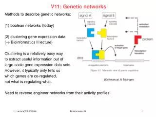
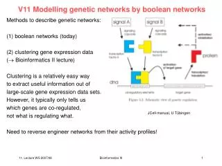
V11 Modelling genetic networks by boolean networks Methods to describe genetic networks: (1) boolean networks (today) (2) clustering gene expression data ( Bioinformatics II lecture) Clustering is a relatively easy way to extract useful information out of large-scale gene expression data sets. However, it typically only tells us which genes are co-regulated, not what is regulating what. Need to reverse engineer networks from their activity profiles! JCell manual, U Tübingen Bioinformatics III
Boolean networks Boolean networks allow dynamic modelling of synchronous interactions between vertices in a network. They belong to the simplest models that possess some of the biological and systemic properties of real gene networks. In Boolean logic, a Boolean variable x is a variable that can assume only two values. The values are denoted usually as 0 and 1, and correspond to the logical values true and false. The logic operators and, or, and not are defined to correspond to the intuitive notion of truthfulness and composition of those operators. A Boolean function is a function of Boolean variables connected by logic operators. Bioinformatics III
Boolean networks A Boolean network is a directed graph G(X,E), where the vertices, xi X, are Boolean variables. To each vertex, xi, is associated a Boolean function, b(xi1, xi2, …, xil) , l n, xij X, where the arguments xj are limited to the parent vertices of xiin G. Together, at any given time, the values of all vertices represent the state of the network, given by the vector S(t) =(xi1(t), xi2(t), …, xilt)). For gene networks, the vertex variables correspond to levels of gene expression, discretized to either 0 or 1. The Boolean functions at the vertices model the aggregated regulation effect of all their parent vertices. The states of all nodes are updated at the same time according to their respective Boolean functions: Bioinformatics III
Boolean networks The transitions of all states together correspond to a state transitionof the network from S(t) to the new network state, S(t+1). A series of state transitions is called a trajectory. Since there is a finite number of network states, all trajectories are periodic. This simply follows from the fact that as soon as one state is visited a second time, the trajectory will take exactly the same path as for the first time. The repeating parts of the trajectories are called attractors, and can be one or more states long. All the states leading to the same attractor are the basin of attraction for this attractor. Bioinformatics III
Reverse engineering Boolean Networks Clustering is a relatively easy way to extract useful information out of large-scale gene expression data sets. However, it typically only tells us which genes are co-regulated, not which gene is regulating what other gene(s). The goal in reverse engineering Boolean networks is to infer both the underlying topology (i.e. the edges in the graph) and the Boolean functions at the vertices from observed gene expression data. The actual observed data can come either from gene expression experiments conducted at different time intervals or when the expression of various genes is perturbed. For time-course data, measurements of the gene expressions at two consecutive time points simply correspond to two consecutive states of the network, S(i) and S(i+1). Bioinformatics III
Intergenic interaction matrix M Perturbation data come in pairs, which can be thought of as the input/output states of the network, Ii/Oi, where the input state is the one before the perturbation and the output the one after it. Given the observations of the states of a Boolean network, in general many networks may be constructed that are consistent with that data. Hence the solution network is ambiguous. There are several variants of the reverse engineering problem: (a) finding one network consistent with the data, (b) finding all networks consistent with the data, and (c) finding the 'best' network consistent with the data (according to some pre-specified criteria). The first task is the simplest one and efficient algorithms exist. Bioinformatics III
Reverse engineering of boolean networks The reverse engineering problems are intimately connected to the amount of empirical data available. Obviously, the inferred network will be less ambiguous the more data points are available. The amount of data needed to completely determine a unique network is known as the data requirement problem in network inference. The amount of data required depends on the sparseness of the underlying topology and the type of Boolean functions allowed. This can be understood intuitively. A network with few connections may be defined with few data points. In the worst case, the deterministic inference algorithms need on the order of m = 2ntransition pairs of data (experimental data points) to infer a densely connected Boolean Network with general Boolean functions at the n vertices. Aracena & Demongeot, Acta Biotheoretica 52, 391 (2004) Bioinformatics III
Intergenic interaction matrix M Since introducing the detection of gene expression by microarrays, a major problem has been the estimation of the intergenic interaction matrix M. In V10, the entries of M were either 0 or 1. Today, we allow the matrix element mijof the interaction matrix M to be - positive if gene Gjactivates gene Gi - negative if gene Gjinhibits gene Gi - equal to 0 if gene Gjand gene Gi have no interaction. Bioinformatics III
simulating the dynamics of regulatory networks Given the interaction matrix M, the change of state xi of gene Gibetween t and t +1 obeys a threshold rule: where H is the Heavyside function H(y) = 1 if y 0 and H(y) = 0 if y < 0, and the bi‘s are threshold values. In the case of small regulatory genetic systems, the knowledge of such a matrix M makes it possible to know all possible stationary behaviors of the organisms having the corresponding genome. Aracena & Demongeot, Acta Biotheoretica 52, 391 (2004) Bioinformatics III
Example In the genetic regulatory network which rules Arabidopsis thaliana flower morphogenesis (right), the interaction matrix is a (11,11) matrix with only 22 non zero coefficient. Below: A fixed configuration (attractor) of its Boolean dynamics that is obtained from propagating xi(t). Mendoza, Alvarez-Buylla, JCB, 1998 Bioinformatics III
Reverse engineering of the interaction matrix For each genetic regulatory network, we can define an interaction graph built from the interaction matrix M by drawing an edge + (resp. -) between the vertices representing the genes j and i, iff mij > 0 (resp. < 0). To calculate the mij´s, we can either determine the s-directional correlation ij(s) between the state vector {xj(t – s)}t C of gene j at time t – s and the state vector {xi(t)}t C of gene i at time t , t varying during the cell cycle C of length K = | C | and corresponding to the observation time of the bio-array images: Aracena & Demongeot, Acta Biotheoretica 52, 391 (2004) Bioinformatics III
interaction matrix and then take where is a de-correlation threshold. Alternatively, one may identify the system with a Boolean neural network. When it is impossible to obtain all the coefficients of M in this manner (either from the literature or from such calculations), it may be possible to complete M by appyling an heuristic approach. Aracena & Demongeot, Acta Biotheoretica 52, 391 (2004) Bioinformatics III
estimation of interaction values We may randomly choose the missing coefficients by considering - the connectivity coefficient K(M) = I / N, the ratio between the number I of interactions and the number N of genes, and - the mean inhibition weight I(M) = R / I , the ratio between the number of inhibitions R and I. For many known operons and regulation networks, K(M) is between 1.5 and 3, and I(M) between 1/3 and 2/3. If M is structurally stable, then the random estimation of M can be used to obtain an approximate estimation on the control mechanisms of the regulatory network. Aracena & Demongeot, Acta Biotheoretica 52, 391 (2004) Bioinformatics III
Monod and Jacob (1961) first proposed that complex networks of gene interactions regulate cell differentiation. The first formal models of genetic regulation of cell differentiation anticipated that real biological genetic networks would be too complex to be analyzed without the use of formal mathematical and/or computational tools. However, because the early models made some assumptions that were biologically unrealistic, experimentalists largely ignored them. Relatively complete genetic descriptions of developmental programs are now available in several model organisms, providing the necessary inputs for developing biologically realistic dynamic models of gene regulatory networks in cell differentiation. Such models should aid at building a formal framework for studies of developmental mechanisms and their evolution. Espinosa-Soto et al. The Plant Cell 16, 2923 (2004) Bioinformatics III
methods The model is discrete. N is the number of genes involved in the network, Xn is a vector with expression state for each gene in a space of N dimensions, representing the network state after n iterations: where xi(n) represents the state of expression of the gene i at the iteration n. We then write: indicating that the state at the iteration (n + 1) is determined by the state at the previous iteration. Each node, except SEP (redundant SEP1, SEP2, and SEP3 genes), stands for the activity of a single gene involved in floral organ fate determination. Most nodes could assume three levels of expression (on, 1 or 2, and off, 0) to enable different activation thresholds when experimental data was available. Espinosa-Soto et al. The Plant Cell 16, 2923 (2004) Bioinformatics III
functions of genes inferred from experiments FLOWERING LOCUS T Double embryonic flower1 (emf1) flowering locus t (ft) mutants do not develop embryonic flowers typical of emf1 single mutants, suggesting that the lack of FT activity suppresses the emf1 phenotype because EMF1 represses FT. LFY Double mutants of the weak emf1-1 allele and lfy-1 bear lfy-like flowers, suggesting that, for this trait, lfy is epistatic. These genes have antagonistic activities; hence, we infer that LFY is repressed by EMF1. TFL1 In emf1-2 tfl1 double mutants, the emf1-2 mutation is epistatic. As these two genes do not have opposite functions, this result suggests that EMF1 protein is needed for TFL1 activity in wild-type Arabidopsis. .... Espinosa-Soto et al. The Plant Cell 16, 2923 (2004) Bioinformatics III
logical rules Espinosa-Soto et al. The Plant Cell 16, 2923 (2004) Bioinformatics III
logical rules Espinosa-Soto et al. The Plant Cell 16, 2923 (2004) Bioinformatics III
logical rules Espinosa-Soto et al. The Plant Cell 16, 2923 (2004) Bioinformatics III
network architecture Figure 4. Gene Network Architecture for the Arabidopsis Floral Organ Fate Determination. Network nodes represent active proteins of corresponding genes, and the edges represent the regulatory interactions between node pairs (arrows are positive, and blunt-end lines are negative). Dashed lines are hypothetical interactions for which there is no experimental support (see logical rules). The network includes F-box proteins (UFO), membrane bound signaling molecules (TFL1 and FT), cofactors involved in transcriptional regulation (EMF1 and LUG), chromatin remodeling proteins (CLF), and transcription factors (all others). Interactions have been confirmed to be direct transcriptional regulations in a few cases (LFY on AG, LFY on AP1), and the rest can either be direct or indirect and can be transcriptional or other. Espinosa-Soto et al. The Plant Cell 16, 2923 (2004) Bioinformatics III
states of the system The system has a finite number of possible initial conditions equal to 139,968, and each one is represented by a vector of dimension 15 in which each column corresponds to the expression state of each network node at initial conditions in the following order: FT EMF1 TFL1 LFY FUL AP1 AP3 PI AG UFO WUS AP2 SEP LUG CLF. The vector of 15 entries that keeps track of the activity level of each node describes the system at each time point. We updated the state of each node synchronously. Starting on each initial condition the network is iterated until it reached an attractor. The 139,968 initial states converge to only 10 stable attractors. All of them are fixed point attractors in which the activity level of all genes remains the same as in the previous iteration, see table 1. Espinosa-Soto et al. The Plant Cell 16, 2923 (2004) Bioinformatics III
simulated gene expression levels These steady gene states (Table 1) predicted by the model coincide with the gene expression profiles that have been documented experimentally in cells of wild-type Arabidopsis inflorescence meristems and floral organ primordia. For example, in the Infl steady states, floral meristem identity genes (LFY, AP1, and AP2) and floral organ identity genes (AP1, AP2, AP3, PI, SEP, and AG) are off, whereas the inflorescence identity genes (EMF1 and TFL1) are on. Espinosa-Soto et al. The Plant Cell 16, 2923 (2004) Bioinformatics III
attractors The size of the basins of attraction may indicate how stable each morphogenetic response is and which genes are critical to attain each cell fate Espinosa-Soto et al. The Plant Cell 16, 2923 (2004) Bioinformatics III
petunia gene network Deciphering network architectures underlying cell differentiation is a first step toward understanding the mechanisms that rule conservation and variation in morphological traits. Although most flowering species have an overall conserved plan of floral organ determination, mutations have revealed some important variations. In the case of petunia, the overall network of cell fate determination during flower organ development seems to be conserved with respect to Arabidopsis. However, mutant analyses have suggested some differences. Our simulation results suggest that an architecture like the one proposed here for the Arabidopsis network that includes a duplicated AP3 would yield the gene expression patterns observed for the wild type and a single AP3-like gene mutant and provides a prediction for the double loss-of-function mutations of AP3-like genes in petunia. Espinosa-Soto et al. The Plant Cell 16, 2923 (2004) Bioinformatics III
comparison arabidopsis - petunia Figure 5. Arabidopsis and Petunia Wild Type (left), ap3 Mutant (right) Flowers, and Corresponding Network Models. Single petunia mutant for PhDEF is shown in the top part of (B) and a scheme of the predicted double mutant for PhDEF and PhTM6 is shown below. Arabidopsis is shown in (A). The networks indicate which nodes were turned off (yellow) to simulate mutants. The Arabidopsis orthologs of the cloned petunia genes are as follows: FLORAL BINDING PROTEIN26 (FBP26) is an AP1 ortholog, PhDEF (formerly known as GREEN PETALS) is an AP3 and DEFICIENS (DEF; from A. majus) ortholog, PhGLO1 (FBP1) and PhGLO2 (PETUNIA MADS BOX GENE2; pMADS2) are PI and GLOBOSA (GLO; from A. majus) orthologs, pMADS3 is an AG ortholog, PhAP2A is an AP2 ortholog, FBP2 and FBP5 are SEP orthologs, PhCLF1 and PhCLF2 are CLF orthologs, and PETUNIA HYBRIDA TM6 (PhTM6) is a paleoAP3 gene. Espinosa-Soto et al. The Plant Cell 16, 2923 (2004) Bioinformatics III
comparison arabidopsis - petunia Espinosa-Soto et al. The Plant Cell 16, 2923 (2004) Bioinformatics III
Control of Gene Expression A bacterial cell lives in direct contact with its environment. Its chemical composition may dramatically change from one moment to the other. Consider bacteria growing either on lactose or tryptophan. Fig. 2.16 Lactose: di-saccharide from glucose + galactose oxidation provides cells with metabolic intermediates and energy. First step of lactose degradation (catabolism): hydrolysis of the bond joining the 2 sugars by -galactosidase [Karp] Cell & Mol. Biol. Bioinformatics III
Transfer from minimal medium to lactose medium When bacterial cells are grown in a minimal medium, they don‘t need -galactosidase and contain < 5 copies and only 1 copy of its mRNA. What happens when the cells are transferred to a lactose medium? [Karp] Cell & Mol. Biol. Bioinformatics III
lac Operon: an inducible operon Inducible operon: presence of substance (lactose) induces transcription of the structural genes. lac operon contains 3 tandem structural genes: z gene: encodes -galactosidase y gene: encodes galactoside permease, a protein that promotes entry of lactose into the cell a gene: encodes thiogalactoside acetyltransferase [Karp] Cell & Mol. Biol. Bioinformatics III
positive control by cyclic AMP Repressors, such as those of the lac and trp operons, exert their influence by negative control. lac operon is also under positive control, the „glucose effect“. If bacterial cells are supplied with glucose (as well as with other substances such as lactose or galactose), the cells catabolize the glucose and ignore the other compounds. glucose in the medium suppresses the production of various catabolic enzymes, such as -galactosidase, needed to degrade the other substrates. In 1965, cAMP was deteced in E.coli. The higher the glucose concentration, the lower the cAMP concentration. When adding cAMP to the medium in the presence of glucose, the catabolic enzymes that were normally absent were suddenly synthesized by the cell. cAMP binds to CRP. The cAMP-CRP complex recognizes and binds to a specific site in the lac control region. The presence of bound CRP changes the DNA conformation and allows RNA polymerase to transcribe the lac operon. [Karp] Cell & Mol. Biol. Bioinformatics III
positive control by cyclic AMP Fig. 12.27 [Karp] Cell & Mol. Biol. Bioinformatics III
Growth on Trp medium Trp is required for protein synthesis. If no Trp is available in the medium, the bacterium must expend energy synthesizing this amino acid cells contain enzymes and corresponding mRNA of Trp-synthesis pathway. If Trp becomes available in the medium, the cells no longer have to synthesize their own Trp. Within a few minutes, the production of the enzymes of the Trp pathway stops. In the presence of Trp, the genes encoding these enzymes are repressed. [Karp] Cell & Mol. Biol. Bioinformatics III
trp operon In a repressible operon, the repressor is unable to bind to the operator DNA itself. [Karp] Cell & Mol. Biol. Bioinformatics III
eukaryotic gene expression: PEPCK model case: gene that codes for phosphoenolpyruvate carboxykinase (PEPCK). This enzyme is one of the key enzymes of gluconeogenesis, the metabolic pathway that converts pyruvate to glucose. The enzyme is synthesized in the liver when glucose levels are low, e.g. when considerable time has passed since your last meal. Synthesis drops sharply after carbohydrate-rich meal. Level of synthesis of PEPCK mRNA is controlled by a variety of transcription factors, including several hormone receptors that are involved in regulating carbohydrate metabolism. To understand the regulation of PEPCK gene expression, we need to (1) unravel the functions of the numerous DNA regulatory sequences that residue upstream from the gene itself (2) identify the transcription factors that bind these sequences, and (3) identify the signalling pathways that activate the machinery responsible for selective gene expression. [Karp] Cell & Mol. Biol. Bioinformatics III
eukaryotic gene expression: PEPCK Fig. 12.32 TATA box followed by core promoter: site of assembly of a pre-initiation complex consisting of RNA polymerase II and a number of general TFs CAAT + GC boxes: bind global TFs such as NF1 and SP1; both are typically located 100 – 150 bp upstream proximal promoter elements [Karp] Cell & Mol. Biol. Bioinformatics III
Responsive elements from PEPCK gene various hormones affect the expression of PEPCK gene: insulin, thyroid hormone, glucagon, glucocorticoid. All of the act by means of specific TFs that bind to the DNA. Fig. shows responsive elements. [Karp] Cell & Mol. Biol. Bioinformatics III
Activation of transcription For example, let us focus on glucocorticoids, a group of steriod hormones (e.g. cortisol) that are synthesized in response to stress. Fig. 12.34 [Karp] Cell & Mol. Biol. Bioinformatics III
Conservation of regulatory elements? Nature 423, 241 (2003) Bioinformatics III
Comparative genome analysis Compare sequences of Saccharomyces paradoxus, S. mikatae, S. bayanus, with S. cerevisae. The three new yeast species have sufficient sequence similarity to S. cerevisiae to allow orthologous regions to be aligned reliably, but sufficient sequence divergence to allow many functional elements to be recognized by their greater degree of conservation by a four-way species comparison. Assemble with Arachne program Align 4 genomes. Nature 423, 241 (2003) Bioinformatics III
Conservation of the Gal4-binding site We first studied the binding site for one of the best-studied transcription factors, Gal4, whose sequence motif is CGGn(11)CCG (which contains 11 unspecified bases). Gal4 regulates genes involved in galactose metabolism, including the GAL1 and GAL10 genes, which are divergently transcribed from a common intergenic region. The Gal4 motif occurs three times in this intergenic region, and all three instances show perfect conservation across the four species. In addition, there is a fourth experimentally validated binding site for Gal4 that differs from the consensus by one nucleotide in S. cerevisiae. This variant site is also perfectly preserved across the species. Nature 423, 241 (2003) Bioinformatics III
Conservation of the Gal4-binding site We then examined the frequency and conservation of Gal4-binding sites across the aligned genomes. In S. cerevisiae, the Gal4 motif occurs 96 times in intergenic regions and 415 times in genic (protein-coding) regions. The motif displays certain marked conservation properties: (1) occurrences of the Gal4 motif in intergenic regions have a conservation rate (proportion conserved across all four species) that is about fivefold higher than for equivalent random motifs. (2) intergenic occurrences of the Gal4 motif are more frequently conserved than genic occurrences. By contrast, random motifs are less frequently conserved in intergenic regions than in genic regions, reflecting the lower overall level of conservation in intergenic regions. Thus, the relative conservation rate in intergenic compared with genic regions is about 11-fold higher for Gal4 than for random motifs. (3) the Gal4 motif shows a higher conservation rate in divergent compared with convergent intergenic regions (those that lie upstream compared with downstream of both flanking genes); no such preferences are seen for control motifs. These three observations suggest various ways to discover motifs based on their conservation properties. Nature 423, 241 (2003) Bioinformatics III
Assign function Assign candidate functions to these discovered motifs by the genes adjacent to conserved occurrences of the motif with known gene categories. Test for Gal4 motif. Given the biological role of Gal4, we considered the set of genes annotated to be involved in carbohydrate metabolism (126 genes according to the Gene Ontology classification) with the set of genes that have a Gal4-binding motif upstream. The intergenic regions adjacent to carbohydrate metabolism genes comprise only 2% of all intergenic regions, but 7% of the occurrences of the Gal4 motif in S. cerevisiae and 29% of the conserved occurrences across the four species. suggests that a function of the Gal4 motif could be inferred from the function of the genes adjacent to its conserved occurrences. Such putative functional assignments can be useful in directing experimentation for understanding the precise function of a motif. Such considerations indicate that it should be possible to use comparative analysis, such as explored here for yeast, to identify directly many functional elements in the human genome that are common to mammals. More generally, comparative analysis offers a powerful and precise initial tool for interpreting genomes. Nature 423, 241 (2003) Bioinformatics III