Download
1 / 46
460 likes | 703 Views
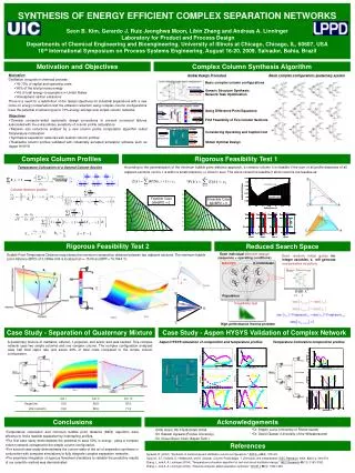
Synthesis and Optimization of Separation Sequence. Libin Zhang and Andreas A. Linninger Laboratory for Product and Process Design , Department of Chemical Engineering, University of Illinois, Chicago, IL 60607, U.S.A. A. AB. ABC. B. BC. ABCD. ABCDE. BCD. C. BCDE. CD. CDE. D.

E N D
Synthesis and Optimization of Separation Sequence Libin Zhang and Andreas A. Linninger Laboratory for Product and Process Design, Department of Chemical Engineering, University of Illinois, Chicago, IL 60607, U.S.A.
A AB ABC B BC ABCD ABCDE BCD C BCDE CD CDE D DE E Motivation P1 Which SEPARATION configuration is optimal???? PURITY SPECIFICATIONS XA = 0.99, Xb = 0.001,…. X2 P2 FEED Components: A,B, C,D,E Known Compositions X1 P3 Maximum profitand/or Minimum environmental impact X3 P4 X4 structure and operating conditions P5
Outline • Long-term objectives: “Computational synthesis of separation networks” • Algorithmic Approach to determine feasibility of separation specification • Methodology - Minimum Bubble Point Distance Algorithm (MIDI) • Assessing Feasibility of given Separation Tasks • Feasible Range of Column Operations: Minimum & Maximum Refluxes • Toward Computed Aided Distillation Synthesis • Feasibility Test +Genetic algorithm (Stochastic search) • Temperature collocation on finite element • Reduced search space, but rigorous models (non-ideal separations) • Genetic algorithm and feasibility test • Infeasible path algorithm
Quick and Reliable Feasibility Test PRODUCT A PURITY SPECIFICATIONS XA = 0.99, Xb = 0.001,…. SIMPLE DISTILLATION COLUMN ? FEED Components: A,B, C Known Compositions PRODUCT B SEPARATION TASK FEASIBLE????
1.6 F 50 1.2 Solution Approaches 1. SIMULATION APPROACH 2. DESIGN APPROACH • Performance Calculation • Flowsheet Simulator • Aspen Plus, HYSYS, Pro/II • Design Calculation • Given Feed & 4 D.O.F • SPECIFICATION FEASIBLE?? ??? Given XA,D XB,D DISTILLATE F Fixed Trays ?? Reflux Given Feed Given Feed Given XA,B ??? BOTTOMS • Trial and Error Approach • Does not Assess Feasibility • Direct Feasibility assessment • Evaluate Column Profiles
x2 Feed x1 Design Approach - Underwood’s Equations NUMERICAL PROBLEM ?? OR INFEASIBLE SPECIFICATION?? • Underwood’s Equations • Highly Non-Linear • Difficult to Converge Rectifying Equations (1) Stripping Equations (2) Profile Intersection: (3)
A Robust Column Design Algorithm • Main ideas • 1. Model Column Profile: • Temperature (Not Trays) • Continuous Profile Equations (Doherty, 1985) • 2. Feasibility Check: • Minimum Bubble Point Distance between Rectifying & Stripping Profiles • 3. Solution Strategy • Finite Element Collocation on Orthogonal Polynomials • Supporting Concepts • Pinch Point • Attainable Temperature Window • Bubble Point Distance
x2 d x1 Reachable Temperatures - Pinch Points • Fixed points in the composition profiles • Pinch, saddle and unstable points • Newton-Horner (Deflation), Continuation Method, Bounded Newton-Raphson algorithm d: distillation : unstable point : saddle point : pinch point (OL) (EQ) At the pinch point: Let in equilibrium withxi,p Pinch equation: Residual Error d (PL) Temperature, ºF
B P2 Temperature x2 P1 P1 TBottoms Infeasible column Feed B D B Temperature p2 NO OVERLAP x1 Attainable Temperature Window P2 D p1 P2 D P1 TDistillate If , column is infeasible Attainable Temperature Window • Difference between boiling points and the stable points of rectifying and stripping section
TB TA x2 dB dA x1 (3) (1) (2) Acetaldehyde Methanol Water Bubble Point Distance • Bubble Point Distance: • The Euclidean difference of two points on the rectifying and stripping profile whose BP is equal to T; • Feasibility test: p1, p2; p1rectifying ; p2 stripping; (BPD(p1, p2)) Feasible Min d = 0 Infeasible d > 0 T d
d Infeasible Case Feasible Case d Log(x3) Point of feasible specification Xd3=0.0005, =0.36 2. Minimum Bubble Point Distance(MIDI) Dimensionless Temperature: s.t.
n+1 n Modeling Column Profile:Continuous Differential Equation (Doherty, 1985) • Continuous differential equation for evolution of column profile (Doherty,1985) • Taylor expansion truncated after first term Continuous column profile with independent variable h Stripping Section: Eq. (1) Rectifying Section: Eq. (2)
Temperature Collocation of Column Profiles • Temperature is monotonically increasing in distillation column (normally) • Temperature is bounded : from Distillate and Bottom temperature to the pinch points Implicit Differentiation Eq. (3) Stripping profile: Eq. (4) Rectifying profile: Eq. (5)
x Polynomials · x3[i]= x0[I+1] · · 0th Node Lagrangian polynomials x2[i] · · · x1[i] · x3[I-1]=x0[i] · ´ ´ ´ ´ ´ ´ ´ ´ 1st Node Lagrangian polynomials D P1 Collocation nodes Element 1 Element NS Element i Element i+1 2nd Node Lagrangian polynomials 3th Node Lagrangian polynomials 3. Temperature Finite Element Collocation • Globally collocatge entire profile between two temperatures • Using 3-5 finite elements and 2-3 nodes
Branch of saddle pinches c b Branch of maximum nodes of composition profile c’ a b’ x,Composition a’ Temperature, ºF Element Placement • Saddle temperature place an element boundary at the composition profile • The saddle coincide with maximum curvature of the intermediate species
Application 1: Constant Alpha Mixtures • Compute rectifying profile and stripping profile with pseudo-temperature respectively. • Pseudo Temperature: • Then search the minimum distance between profiles. ATW is not empty But Specification is infeasible MIDI = 0.295 B Feasible MIDI 0 P1 Temperature P2 D Xd1= 0.95;xd2=0.049,xb1=0.05;R= 1.0 Xd1= 0.95;xd2=0.049,xb1=0.05;R=2.5
1.0 0.8 Saddle point Saddle point 0.6 x2 r = 5 x2 r=2.5 0.4 0.2 Feed Distillation Bottoms 1 Methanol 2 Ethanol 3 n-propanol Feed Distillation Bottoms 1 Pentane 2 Hexane 3 Heptane 0.3000 0.9800 5.0•10-4 0.0 0.2500 0.3000 0.3000 0.9500 0.0490 0.0200 0.3513 0.0500 0.3965 0.0 0.2 0.4 0.6 0.8 1.0 Feed x1 x1 0.4500 5.0•10-11 0.6482 0.4000 0.0010 0.5535 Feed (2) (2) (3) (3) (1) (1) Hexane Methanol n-propanol Heptane Pentane Ethanol Application 2: Ideal Mixtures Feasibility test works for both sloppy and sharp split in ideal mixture
(2) (2) (2) B B B (1) (1) (1) A A A (2) (2) (2) (4) (4) (4) Ethanol Ethanol Ethanol D D D (2) (2) (2) Hexane Hexane Hexane (1) (1) (1) Methanol Methanol Methanol (1) (1) (1) Pentane Pentane Pentane (4) (4) (4) Acetic acid Acetic acid Acetic acid (4) (4) (4) Octane Octane Octane Application 3: Quaternary Mixtures Constant alpha mixture Ideal mixture Non-ideal mixture
Random Experiments Random Experiments Random Experiments No. of design specifications No. of design specifications No. of design specifications 10000 10000 10000 No. of feasible designs No. of feasible designs No. of feasible designs 468 533 223 No. of infeasible designs No. of infeasible designs No. of infeasible designs 9532 9777 9463 Convergence failures Convergence failures Convergence failures 0 0 0 Execution time (s) Execution time (s) Execution time (s) 459.8 1017.5 39.4 1.0 (2) (2) (2) Methanol Methanol Methanol 1.0 1.0 0.8 0.8 0.8 0.6 Feed (2) (1) (3) (3) (2) (1) 0.6 0.6 Hexane Pentane Heptane Heptane Hexane Pentane x 0.4 2 0.4 0.4 0.2 0.2 0.2 0.0 0.0 0.2 0.4 0.6 0.8 1.0 0.0 0.0 0.0 0.0 0.2 0.2 0.4 0.4 0.6 0.6 0.8 0.8 1.0 1.0 x (3) (3) (3) (1) (1) (1) 1 Water Water Water Acetaldehyde Acetaldehyde Acetaldehyde Application 4: Feasible Regions Column Specification Search Space (10,000 possibilities) Feasible region Constant alpha 39.4s Feasible region Ideal Mixture Feasible region Non-Ideal Mixture x2 468.8s 1017.5s x1
Feasible Range of Column Operation • Minimum & Maximum Reflux Ratio Calculation • Feasible design: between minimum & maximum reflux ratio RMax x2 RMin Feed x1
Input specification of product and feed (xd and xb) initial guess(rLow, r1,r2, rUp) Compute MIDI r1New =rLow+ r r2New =rLow+ (1-) r No Compute sensitivity (d/r) If feasible r ? Yes Yes If all sign of d/r are same rUp =r, Flag=1 No No If d/r>0 No Yes rUp =r rLow =r rUp - rLow <tol Yes If flag=1 No Yes Output rmin Output infeasible Minimum Reflux Ratio Algorithm • Find the smallest reflux ratio with MIDI0 • Golden Section Search Minimum Reflux Ratio Algorithm
Saddle point x2 rmin=1.36 Feed Distillation Bottoms 1 Methanol 2 Ethanol 3 n-propanol Feed Distillation Bottoms 1 Pentane 2 Hexane 3 Heptane x2 0.3000 0.9800 5.0•10-4 rmin=1.51 0.3000 0.2500 0.3000 0.0200 0.0490 0.9500 0.3513 0.0500 0.3965 x1 0.4500 5.0•10-11 0.6482 0.4000 0.0010 0.5535 Feed Feed (2) (1) (2) (3) (3) (1) x1 Ethanol Pentane Methanol n-propanol Hexane Heptane Minimum Reflux Ratio A reflux specification leading to a zero bubble point distance of rectifying and stripping profiles at stationary pinch point is minimum
(2) (2) (2) Ethanol Ethanol Ethanol Direct Split x2 rmin=1.43 (3) (3) (3) (1) (1) (1) n-propanol n-propanol n-propanol Methanol Methanol Methanol x2 rmin=2.85 Feed x1 x1 Transition Split Feed Feed Feed (3) (2) (1) rmin=1.663 x2 Pentane Heptane Hexane rmin=1.02 x2 x1 x1 Minimum Reflux Ratio: Different Splits Sharp split Indirect Split Minimum Reflux found for sloppy and sharp splits Direct, indirect and transition splits Sloppy splits
1.0 1.0 0.8 0.8 0.6 x2 0.6 rmax=13.01 x2 rmax=9.5 0.4 0.4 Feed Distillation Bottoms 1 Pentane 2 Hexane 3 Heptane Feed Distillation Bottoms 1 Pentane 2 Hexane 3 Heptane 0.2 0.2 0.3000 0.4000 0.4000 0.1000 0.4000 0.0800 0.9100 0.5900 0.0100 0.3430 0.4721 0.0010 0.0 0.5000 0.3000 0.0100 0.0100 0.6470 0.5269 0.0 0.2 0.4 0.6 0.8 1.0 x1 0.0 0.0 0.2 0.4 0.6 0.8 1.0 x1 Feed Feed (1) (2) (2) (1) (3) (3) Pentane Heptane Heptane Hexane Pentane Hexane Maximum Reflux Ratio A reflux leading to a zero bubble point distance between rectifying and stripping profiles at bottom or distillate product temperature is maximum.
1.0 1.0 True pinch 0.8 0.8 Close tangent pinch region T T 0.6 0.6 x2 x2 0.4 0.4 P 0.2 0.2 0.0 0.0 0.2 0.4 0.6 0.8 1.0 0.0 0.0 0.2 0.4 0.6 0.8 1.0 x1 x1 (1) (2) (3) (3) (2) (1) Methanol Water Acetaldehyde Methanol Acetaldehyde Water Tangent Pinches In non-ideal mixtures, tangent pinch point controls composition profile. In near tangent pinch situations, MIDI algorithm traverses the region robustly (similar to behavior close to saddle points).
A AB ABC B BC ABCD ABCDE BCD C BCDE CD CDE D DE E Motivation P1 Which SEPARATION configuration is optimal???? PURITY SPECIFICATIONS XA = 0.99, Xb = 0.001,…. X2 P2 FEED Components: A,B, C,D,E Known Compositions X1 P3 Maximum profitand/or Minimum environmental impact X3 P4 X4 structure and operating conditions P5
0 D 1 m F n 1 0 B B Azeotrope F D Challenges • Problem Size of Column Sequences • Large number of state variables (compositions, temperatures,…) • Highly non-linear relationships; • Vapor-liquid equilibrium model • Local convergence • Search for Structural and Parametric Design Variables • Generate structural alternatives • Find optimal parameters without getting trapped in local minima • Converge to global solution in reasonable time; • Solution Approach: • Feasibility test and genetic algorithm • Infeasible path algorithm • Reduced search space and minimum design variable set • Rigorous models
Temperature Collocation Algorithm(Zhang and Linninger, IECR 2004) Coordinate Transformation of Column Profiles into DAE Orthogonal Collocation on Finite Element Bubble points = independent variable BPD (T): Rigorous Feasibility Criterion= : min BPD ~ 0; Infeasible Min bpd > 0 Feasible Min bpd = 0 TB T TA x2 dB dA bpd x1
1.0 1.0 1.0 0.8 0.8 0.6 0.6 0.8 0.4 0.4 0.2 0.2 0.6 0.0 0.0 0.2 0.4 0.6 1.0 0.8 0.0 0.0 0.2 0.4 0.6 0.8 1.0 0.4 0.2 0.0 0.0 0.2 0.4 0.6 0.8 1.0 (1) (3) (1) (3) (2) (2) Benzene Benzene Acetone Chloroform Chloroform Acetone Temperature Collocation Algorithm-Results(Zhang and Linninger, 2004) • Column Profiles = DAE • 10,000 specifications in 39.4 CPUs • Robust Convergence for feasible and infeasible specification 10,000 random specifications 39.4 s for finding all feasible specs Azeotropes/ non-ideal mix. s.t.
1.0 1.0 OCFE result 0.8 0.8 Hysys result OCFE result 0.6 0.6 Hysys result 0.4 x2 x2 0.4 0.2 0.2 0.0 0.0 0.2 0.4 0.6 0.8 1.0 0.0 0.0 0.2 0.4 0.6 0.8 1.0 (3) (2) (1) (1) (2) (3) x1 x1 Hexane Diethyl Ether Benzene Octane Toluene Hexane Temperature Collocation-High Accuracy • Size reduction: ~1 Order of Magnitude • Hysys~600 equation TC-OCFE~50 equations • High Fidelity Results: • Small differences attributable continuous vs, tray-by-tray (1st order appr.) • V-L Equilibrium implementation
F3 F1 B2 B3 B1 F1 Reduced Search Space Minimum set of design Variables Each individual different designs (sequence + operating conditions) MASTER GA Genetic Algorithm K individuals [D] [A] [B][C] Feasibility Test Population State variables dramatically reduced by temperature collocation Feasibility test ([A][B])([C][D]) Feasibility test High performance Inverse problem
P1 P2 F1 A(BC) F2 AB(C) B1 (A)B(C) ABC P3 (A)BC (AB)C Problem Representation - Column Sequencing Chromosome: • Only products ordered by relative volatility • Mass flowrate in product of each specie • Structure: Integer string ProductI Product II Product III Reflux Structure Encoding Operating Conditions Product Specs
P1 P2 F1 F2 F2 P3 F3 B2 B1 F1 F3 B2 B3 B3 B1 P4 P2 F2 OFFSPRING F1 B2 P4 B1 F3 P3 P1 B3 Crossover Example 2 Patents -> Offspring with parameter and structure variation Mathematical Formulation Operational Parameters’ Crossover Structural Crossover (2) (4) F1 After Crossover, mass balance is still valid (3) (1)
F2 F3 B2 F1 B3 B1 P2 P4 P3 P1 Structural and Parametrical Mutation (2) Operational parameters (4) F1 (3) (1) Integer parameters P1 P2 F1 F2 P3 B1 F3 B2 B3 P4
12 10 8 Cost Function 6 12 4 10 2 0 5 10 15 20 25 30 Generation 8 6 Does not stabilize Does not Convergence 4 2 0 5 10 15 20 25 30 Fitness and Convergence 12 10 Mutation & crossover 8 Cost function Op. Cost + Cap. Cost+ Penalty 6 4 2 0 5 10 15 20 25 30 Generation Crossover without mutation Mutation without crossover Cost function Generation
1.0 1.0 1.0 0.8 0.8 0.8 0.6 0.6 0.6 x2 x2 0.4 0.4 0.4 0.2 0.2 0.2 0.0 0.0 0.0 0.0 0.2 0.4 0.6 0.8 1.0 x1 0.0 0.2 0.4 0.6 0.8 1.0 0.0 0.2 0.4 0.6 0.8 1.0 x1 Initial Population of Ternary Mixture • Different initial population method • Given the composition of all streams • All candidate structure • Only given the composition of products Patterned initial guesses All infeasible designs Random initial guesses
Infeasible Path Approach • Feasible Individual increase at beginning evolution • Trend to stabilize at the end • Optimal Sequences even from all infeasible initial population No of Feasible sequences No of Feasible sequences Generation Generation Only infeasible designs initially
P1 P2 F1 P1 B1 1 Pentane 2 Hexane 3 Heptane F1 D1 P3 1 Pentane 2 Hexane 3 Heptane F1 0.3000 0.3000 0.5221 0.9900 0.0122 0.0063 F2 P1 0.4000 0.4000 0.0027 0.0018 0.9834 0.6375 B1 F2 P3 D1 1.0 1.0 P2 P2 0.3000 0.3000 0.4762 0.0082 0.3503 0.0103 F1 P2 0.8 0.8 P3 0.6 0.6 D1=F2 B1=F2 0.4 0.4 F1 F1 0.2 0.2 P3 P3 P1 P1 0.0 0.0 0.0 0.2 0.4 0.6 0.8 1.0 0.0 0.2 0.4 0.6 0.8 1.0 Case study I: Ideal Ternary Mixture Generation Evolution Min. Cost = 2.56 X10³ Min. Cost = 3.16 X10³
Feed Distillation Bottoms 1 Acetone 2 Chloroform 3 Benzene 0.2000 0.9900 0.0122 0.7000 0.0018 0.6375 0.1000 0.0082 0.3503 (1) (3) (2) Chloroform Benzene Acetone Case study II: Azeotropic Mixture D1(Acetone) 1.0 D2(Chloroform) D2 F1 0.8 F2 II Azeotrope 0.6 B1 I 0.4 B2(Benzene) 0.2 B1 Generation evolution D1 F1 B2 0.0 0.0 0.2 0.4 0.6 0.8 1.0 Penetrate the curved boundary
1.0 0.8 0.6 (2) (3) (1) 0.4 Ethanol Ethylene glycol Water 0.2 0.0 0.0 0.2 0.4 0.6 0.8 1.0 Case study III: Entrainer Azeotropic Separation D2 D1(Ethanol) FUpper D2(Water) F FLower F2 F B2 FLower B3(EG) B1 FUpper D1 Flow sheet for separation of water and ethanol with entrainer Break azeotropic with entrainer
1.0 0.8 R=5.0 0.6 Fr=3.5 Stripping Section 1.0 0.4 D1(Ethanol) 0.8 Middle Section Lower Feed 0.2 FUpper D2(Water) Upper Feed Average Feed M R=4.3 M’ 0.6 Fr=2.14 FLower 0.0 PM 0.0 0.2 0.4 0.6 0.8 1.0 Rectifying Section (2) (1) (3) (2) (3) (1) Stripping Section F2 Water Ethylene glycol Ethanol Water Ethylene glycol Ethanol 0.4 B1 Middle Section Lower Feed 0.2 Upper Feed Average Feed B2(EG) M 0.0 PM 0.0 0.2 0.4 0.6 0.8 1.0 Rectifying Section Case study III: Entrainer Azeotropic Separation Suboptimal solution Best solution
P1 P2 F1 F2 P3 (3) (1) B1 F3 Methanol n-propanol B2 (4) B3 P4 Acetic Acide F3 F1 B2 B3 B1 Case study IV: Quaternary Mixture (2) Ethanol P2 Optimal Cost: 5.98X10³ P4 F1 P1 P3
1.0 P1 Column C1 0.8 0.6 F1 B1 0.4 0.2 P1 1.0 Column C2 B2 0.8 D2 0.6 F2 0.4 B2 0.2 D2 F3 1.0 D2 P2 P3 F1 C3 Column C3 C1 F2 0.8 C1 A(BCDE) C2 F3 (4) (5) (4) (3) (2) (1) (5) (2) (4) (3) (2) (3) (5) 0.6 B1 F4 1-hexanol 1-hexanol 1-octanol 1-heptanol Isobutanol 1-pentanol 1-pentanol 1-heptanol 1-heptanol 1-octanol 1-octanol 1-hexanol 1-pentanol B2 AB(CDE) C4 0.4 F3 (A)B(DE) ABC(DE) 0.2 P2 P3 C3 (A)BC(DE) ABCD(E) 1.0 C3 P4 P5 Column C4 ABCDE C2 (A)BCD(E) (AB)C(DE) F4 0.8 (A)BCDE C1 (AB)CD 0.6 (AB)CDE (ABC)D(E) 0.4 (ABC)DE C4 F4 C2 0.2 C4 P4 P5 (ABCD)E 0.0 480 380 400 420 440 460 Temperature, K Case study V: Five Component Mixture
Conclusion • Minimum bubble point distance algorithm to test feasibility or infeasibility of a design specification. • Profile equation with temperature • Finite element collocation method is used to instead the expensive tray-by-tray model. • Applicability: • sloppy split and sharp split • constant relative volatility, ideal, non-ideal mixtures • multi-component mixtures • Reduced hybrid Algorithm is robust and reliable; • Solution can be obtained from initial population without any feasible point; • Best sequence and operating conditions can be obtained at same time; • Rigorous distillation model -> Necessary for non-ideal and azeotropic mixtures • Reduced Space Genetic Algorithm • Specialized chromosome: mass consistency. • Feasibility Test: massive problem size reduction of state variables