Understanding Image Processing: Techniques and Applications in Digital Signal Processing
This article delves into the fundamentals of image processing, covering critical concepts such as analog and digital signals, quantization, and sampling. It explores visual perception, enhancement techniques, and the significance of contrast and dynamic range in image analysis. By examining practical examples, including color video signals and black-and-white photographs, we highlight the importance of DSP tools used in improving image quality and intelligibility. The discussion also includes histogram modification as a method for enhancing images, providing insights into the transformation processes and analysis techniques.

Understanding Image Processing: Techniques and Applications in Digital Signal Processing
E N D
Presentation Transcript
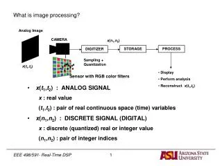
Analog Image CAMERA x(n1,n2) STORAGE PROCESS DIGITIZER Sampling + Quantization x(t1,t2) • Display • Perform analysis • Reconstruct x(t1,t2) What is image processing? • x(t1,t2) : ANALOG SIGNAL x : real value (t1,t2) : pair of real continuous space (time) variables • x(n1,n2) : DISCRETE SIGNAL (DIGITAL) x : discrete (quantized) real or integer value (n1,n2) : pair of integer indices Sensor with RGB color filters 1
Examples • Sampled Black & White Photograph: x(n1,n2) x (n1,n2) scalar indicating piel intensity at location (n1,n2) For example: x = 0 Black x = 1 White 0 < x < 1 In-between • Sampled color video/TV signal xR(n1, n2, n3) xG(n1, n2, n3) xB(n1, n2, n3) 2
Examples 3
How do we process images? • Use DSP concepts as tools • Exploit visual perception properties 4
Visual Perception • We represent pixels as amplitude values (gray scale). 256 levels 1 0 128 levels 1 0 64 levels 1 0 32 levels 1 0 • How much to sample (quantize) the gray scale? • Humans can distinguish in the order of 100 levels of gray (about 40 to 100). 5
Visual Perception: Examples Original image, 8 bits per pixel Processed image, 0.35 bits per pixel 6
Visual Perception RMSE = 8.5 RMSE = 9.0 7
Image Enhancement • Image Enhancement • Objective: accentuate or improve appearance of features, for subsequent analysis or display (possibly, but not necessarily degraded by some phenomenon). • Examples of features: edges, boundaries, dynamic range and contrast. • Examples of applications: • TV: enhance image for viewer (image quality, intelligibility, visual appearance). • Preprocessing for machine identification. • Enhancement is not necessarily needed because of degradation but can be used possibly to remove degradation. 8
Image Enhancement Noise Blurred or faint edges Low contrast or dynamic range Sharpen faint or blurred edges Modify low dynamic range Remove noise 9
Image Enhancement • Types of distortions to correct: • Blur (Blurring due to camera motion, defocusing, …) • Noise (assumed to be additive often for simplicity, although not necessarily the case). • Contrast • Blocking artifacts in block-based transform coders. • Examples: • Space photography • Underwater photography • Film grain noise 10
p(x) Number of occurrences of pixel with a particular intensity x x b a Contrast and Dynamic Range Modification • Contrast stretching • Degradation is commonly due to poor lighting. • Image probability distribution function (pdf) has narrow peak poor contrast. • Image intensities are clustered in a small region available dynamic range is not very well utilized. 11
p(xnew) xnew Contrast and Dynamic Range Modification • Possible solution: increase overall dynamic range • resulting image would appear to have a grater contrast • expand the amplitudes from a to b to cover available intensity range. 12
xnew slope b’ slope a’ a b L x slope Contrast and Dynamic Range Modification • Idea: Gray scale or intensity level of an input image x(n1,n2) is modified according to a specific transformation (function) f(·). • Note: f(·) is usually constrained to be a monotonically non-decreasing function of x ensures that a pixel with higher intensity than another will not became a pixel with a lower intensity in output image xnew. • Typical stretching operator: 13
Contrast and Dynamic Range Modification • Specific desired transformation depends on the application Example: compensation of display non-linearity most suitable transformation depends on display non-linearity. • In most applications, a good or suitable transformation can be identified by computing and analyzing the histogram of the input image to be enhanced. • The histogram is a scaled version of the image pdf. • The histogram gives pdf when scaled by the total number of pixels in the image. 14
normalized Histogram Modification and Equalization • Definition: The histogram of an image h(x) represents the number of pixels that have a specific intensity x number of pixels as a function of intensity x. h(x) = scaled version of pdf p(x) Normalization ensures that 15
hd(xnew) Desired histogram of output image xnew = f(x) xnew Lmin Lmax hi(x) x Histogram Modification and Equalization • Remarks: • Histogram modification methods popular because computing and modifying histogram of an image requires little computations. • Experienced person can easily determine needed transformation by analyzing histogram characteristics. But if too many images automatic method is desired. • For typical natural images, the desired histogram has a maximum around the middle of the dynamic range and decreases slowly as the intensity increases or decreases. • Problem: Determine f(·) such that houtput(xnew) = hd(xnew) 16
hd(x) Redistribute pixels by assigning pixels uniformly to the given levels. const xnew Lmin Lmax pixels assigned to each level Histogram Modification and Equalization • Histogram equalization: special case of histogram modification where hd(x) = constant • For a 256256 image, with 256 intensity levels: • How can we do assignment? 17
16 h(x) 35 35 16 21 21 7 7 1 1 x 0 L1 1 L2 2 L3 3 L4 4 L5 5 L6 6 L7 7 L8 ho(x) 16 16 16 16 16 16 16 16 x 0 L1 1 L2 2 L3 3 L4 4 L5 5 L6 6 L7 7 L8 Histogram Modification and Equalization • Method 1: Collect and redistribute pixels Example: 128 pixels at 8 levels Collect and redistribute pixels. Get bundles of 16 regardless of their position in image. 18
Histogram Modification and Equalization • How to group them? • One approach is to split bins can choose pixels within a bin randomly poor results that tend to be noisy. • Compute average values of neighboring pixels and match to closest average better, but still noisy. • A better approach is to use a cumulative method. 19
hi(xi) ho(xo) xo = f(xi) const xi xo 0 L-1 xmin xmax Histogram Modification and Equalization • Cumulative method for histogram equalization • Histogram equalization desired histogram is constant at all levels. • Problem: Find transformation xo=f(xi) such that that houtput(xo) = const If normalized histogram uniform distribution 20
= normalized histogram = cumulative probability distribution of xi Histogram Modification and Equalization • Solution: • Compute input pdf • Choose • Why? if y uniformly distributed between (0,1) histogram uniformly distributed need also to scale y because y (0,1) instead of (0,L-1) or (Lmin,Lmax) + scaling needed 21
Histogram Modification and Equalization • Note: if y uniformly distributed between (0,1) Proof: 22
only approximately uniformly distributed (because of discretization) Histogram Modification and Equalization • Since xi is a discrete variable, integral is replaced by summation: ymin not necessarily 0 since • Scaling can be done as follows 23
where - rounding operation Histogram Modification and Equalization • If input and output range from 0 to L – procedure can be described as follows: • Procedure: xk = k; k=0,…, L = input amplitude levels yk; k=0,…, L = output amplitude levels • Compute the histogram of the image to be improved. • Normalize histogram; • Normalize amplitudes so that the sum of all values is equal to one and you have a pdf,pi(·). • Compute • Move bins in xk to locations in yk. • Scale yk to desired amplitude range (linear mapping). 24
pi(xk) 0.25 0.25 0.2 0.20 0.15 0.15 0.14 0.1 0.07 0.10 0.05 0.04 0.05 xk; 0≤xk≤7 0 1 2 3 4 5 6 7 Histogram Modification and Equalization • Example: L = 7 Find yk such that xk maps into yk: 25
po(yk) 0.25 0.25 0.25 0.2 0.20 0.16 0.14 0.15 0.10 0.05 0 1 3 5 6 7 Histogram Modification and Equalization yk; 0≤yk≤7 26
Histogram Modification and Equalization Original Image Equalized Image 27
Thresholding • Thresholding can be used to extract objects from image (segmentation) • Histogram statistics can be used to define single or multiple thresholds to classify an image pixel-by-pixel. • A simple approach: • Bimodal histogram set the threshold to gray value corresponding to the deepest point in the histogram value. • Multimodal histogram set thresholds to correspond to points in “valleys” of histogram. • Classify every pixel f(x,y) by comparing its gray level to the selected threshold. 28
Original image Image histogram Thresholded, T=12 Thresholded, T=166 Thresholded, T=225 Pixel-based direct classification methods 29
Thresholding 30