Download
1 / 37
370 likes | 554 Views
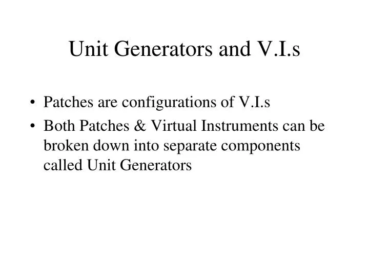
Unit Generators and V.I.s. Patches are configurations of V.I.s Both Patches & Virtual Instruments can be broken down into separate components called Unit Generators. Unit Generators. Have input parameters Have at least one output Perform a function: modification of a signal

E N D
Unit Generators and V.I.s • Patches are configurations of V.I.s • Both Patches & Virtual Instruments can be broken down into separate components called Unit Generators
Unit Generators • Have input parameters • Have at least one output • Perform a function: • modification of a signal • combination of signals
AMP DUR ATTACK TIME DECAY TIME FREQ 1 AMP FREQ 2 MULTIPLIER
AMP FREQ PHASE Oscillators
Oscillators • Can be driven by an algorithm in real time • Computers have, until recently, been too slow to deal with this whilst providing the user with the capabilities they require • So most virtual oscillators use a waveform that is pre-stored in a wavetable
Wavetables • The value of many uniformly placed points on one cycle of a waveform are calculated • These points are stored in a wavetable
Wavetables A pictorial representation of a wavetable; really it’s just a table of numbers 1 0 127 383 255 511 -1
Wavetables • The oscillator will retrieve values from the wavetable to produce the wave • The position we are at along the wave is known as the phase
Phase • The phase of the wave is it’s position in the wave cycle • Normally measured in degrees (0 - 360) or radians • Here it is measured in sample points • Phase (Φ) of 0 is the first sample
Phase • So if the wavetable has 512 sample points • And the phase is 180 • What sample point are we at?
Phase of 180 1 0 127 383 255 511 -1
Periodic Waves • We only store one cycle of the wave because the wave is ‘periodic’ • This means it repeats forever
Wrap Around • So if we talk about a given phase Φ1 Φ1 = 515 • The sample point (Φ) we are looking for in our wavetable is: Φ = Φ1 – 512 = 3
Digital Waves & Sampling Frequency • Sound waves held digitally are cut up into small pieces (or samples) • The number of samples they are cut into affects the smoothness of the wave • CD sampling frequency = 44,100 samps/sec
Wave Playback • Playing back the wave in the wavetable will produce a sound of a particular frequency • Before the wave is played back it must be calculated and then stored • The number of samples used to store each second of the waveform is known as the sampling frequency, fs
Wave Playback • When the wave is played back it is played back at the same sampling frequency, fs • It is possible to figure out the frequency of the wave stored by performing a calculation
Calculating the Frequency of the Wave Held in the Wavetable fs / N = f0 samples per second / samples per cycle = cycles per second (seconds/samples) / (cycles/samples) = (seconds/cycles)
Calculating the Frequency of the Wave Held in the Wavetable fs / N = f0 44,100/512 = 86.13 Hz
Sampling Increment (S.I.) • We don’t just want 86.13Hz • We want any frequency we want • So we use a Sampling Increment
Sampling Increment (S.I.) • The sampling increment is the amount added to the current phase location before the next sample is retrieved and played back • By altering the S.I. we can use the wavetable to create waves of different frequencies
Sampling Increment (S.I.) • Playing back the wave at 86.13Hz means playing it back as it is • This means adding 1 to each phase location before retrieving the next sample and playing it back • This happens 44,100 times a second, and produces 86.13 cycles each second (because there are 512 samples per cycle)
Sampling Increment (S.I.) 44,100/ 512 * 1 = 86.13 Hz fs / N * S.I. = f0
Increasing Playback Frequency • Increasing the S.I. decreases the number of samples played back • So the speed of the wave playback is increased, as is the frequency of the wave produced
S.I. = 2 fs / N * S.I. = f0 44,100/ 512 * 2 = 172.27 Hz
Rearrange the Equation fs / N * S.I. = f0 S.I. = N * f0 / fs
Playback Wave at 250 Hz S.I. = N * f0 / fs S.I. = 512 * 250 / 44,100 = 2.902
Table Look-Up Noise • We only have 512 samples in our wavetable • The points we have samples for may not line up with the points at which we wish to obtain samples • The S.I. is 2.902 but (going from 0) we only have samples at 2 & 3
Dealing With Real Numbers • The samples we want to grab don’t exist! • Options: • truncate: 2.902 becomes 2 • round: 2.902 becomes 3 • or interpolate...
Interpolation • 2.902 is used as the S.I. • so take a value at the initial phase (say 3) • add 2.902 to the initial phase = 5.902 to get the place to take the next value • add 2.902 to this to get the place to take the next value = 8.804 • and so on
0.7 0.3 5.902... 5 6 Interpolation • we don’t have values at these points so we calculate estimated values using the nearest samples (this is interpolation) 0.902 * 0.3 + 0.098 * 0.7 , or 90.2% of 0.3 + 9.8% of 0.7 0.2706 + 0.0686 = 0.3392
Interpolation • Occurs for every sampling increment, so 44,100 times per second • Uses a LOT of processing power • The interpolation process still requires us to round numbers up or down, and so still produces error
Table Look-Up Noise • So rounding is required whatever, and that produces error • This error is known as table look-up noise • This error affects signal to noise ratio (S.N.R.)
S.N.R. • Affects the ratio achievable between quiet and loud sounds. • Dodge (1997): Ignoring the quantisation noise contributed by data converters a 512 entry table would produce tones no worse than 43, 49, and 96 dB SNR for truncation, rounding and interpolation respectively. And a 1024 entry table would produce tones no worse than 109 dB SNR for an interpolating oscillator.”
A Sine Wave time, t 1.5 1 0.5 v(t) 0 -0.5 -1 -1.5 0 T/2 T 3T/2
A Sawtooth Wave 1.5 1 0.5 v(t) 0 -0.5 -1 -1.5 0 T 2T time, t
A Square Wave 1.5 1 0.5 v(t) 0 -0.5 -1 -1.5 0 T/2 T 3T/2 time, t
A Triangle Wave 1.5 1 0.5 v(t) 0 -0.5 -1 -1.5 0 T 2T time, t