Download
1 / 74
760 likes | 1.17k Views
Bayesian Methods with Monte Carlo Markov Chains II. Henry Horng-Shing Lu Institute of Statistics National Chiao Tung University hslu@stat.nctu.edu.tw http://tigpbp.iis.sinica.edu.tw/courses.htm. Part 3 An Example in Genetics. Example 1 in Genetics (1).

E N D
Bayesian Methods with Monte Carlo Markov Chains II Henry Horng-Shing Lu Institute of Statistics National Chiao Tung University hslu@stat.nctu.edu.tw http://tigpbp.iis.sinica.edu.tw/courses.htm
Example 1 in Genetics (1) Two linked loci with alleles A and a, and B and b A, B: dominant a, b: recessive A double heterozygote AaBb will produce gametes of four types: AB, Ab, aB, ab A a b B A b a A a A a B b B B b F (Female) 1- r’ r’ (female recombination fraction) M (Male) 1-r r (male recombination fraction) 3 3
Example 1 in Genetics (2) r and r’ are the recombination rates for male and female Suppose the parental origin of these heterozygote is from the mating of . The problem is to estimate r and r’ from the offspring of selfed heterozygotes. Fisher, R. A. and Balmukand, B. (1928). The estimation of linkage from the offspring of selfed heterozygotes. Journal of Genetics, 20, 79–92. http://en.wikipedia.org/wiki/Geneticshttp://www2.isye.gatech.edu/~brani/isyebayes/bank/handout12.pdf 4 4
Example 1 in Genetics (4) Four distinct phenotypes: A*B*, A*b*, a*B* and a*b*. A*: the dominant phenotype from (Aa, AA, aA). a*: the recessive phenotype from aa. B*: the dominant phenotype from (Bb, BB, bB). b* : the recessive phenotype from bb. A*B*: 9 gametic combinations. A*b*: 3 gametic combinations. a*B*: 3 gametic combinations. a*b*: 1 gametic combination. Total: 16 combinations. 6 6
Example 1 in Genetics (6) Hence, the random sample of n from the offspring of selfed heterozygotes will follow a multinomial distribution: 8 8
Bayesian for Example 1 in Genetics (1) • To simplify computation, we let • The random sample of n from the offspring of selfed heterozygotes will follow a multinomial distribution:
Bayesian for Example 1 in Genetics (2) • If we assume a Dirichlet prior distribution with parameters: to estimate probabilities for A*B*, A*b*,a*B* and a*b* . • Recall that A*B*: 9 gametic combinations.A*b*: 3 gametic combinations. a*B*: 3 gametic combinations. a*b*: 1 gametic combination.We consider
Bayesian for Example 1 in Genetics (3) • Suppose that we observe the data of y = (y1, y2, y3, y4) = (125, 18, 20, 24). • So the posterior distribution is also Dirichlet with parameters D(134, 21, 23, 25) • The Bayesian estimation for probabilities are: =(0.660, 0.103, 0.113, 0.123)
Bayesian for Example 1 in Genetics (4) • Consider the original model, • The random sample of n also follow a multinomial distribution: • We will assume a Beta prior distribution:
Bayesian for Example 1 in Genetics (5) • The posterior distribution becomes • The integration in the above denominator, does not have a close form.
Bayesian for Example 1 in Genetics (6) • How to solve this problem? Monte Carlo Markov Chains (MCMC) Method! • What value is appropriate for
? Lose Lose Win Lose Monte Carlo Methods (1) • Consider the game of solitaire: what’s the chance of winning with a properly shuffled deck? • http://en.wikipedia.org/wiki/Monte_Carlo_method • http://nlp.stanford.edu/local/talks/mcmc_2004_07_01.ppt Chance of winning is 1 in 4!
Monte Carlo Methods (2) • Hard to compute analytically because winning or losing depends on a complex procedure of reorganizing cards • Insight: why not just play a few hands, and see empirically how many do in fact win? • More generally, can approximate a probability density function using only samples from that density
f(x) X Monte Carlo Methods (3) • Given a very large set X and a distribution f(x) over it. • We draw a set of N i.i.d. random samples. • We can then approximate the distribution using these samples.
Monte Carlo Methods (4) • We can also use these samples to compute expectations: • And even use them to find a maximum:
Monte Carlo Example • , find • Solution: • Use Monte Carlo method to approximation
Numerical Integration (1) • Theorem (Riemann Integral): If f is continuous, integrable, then the Riemann Sum: • http://en.wikipedia.org/wiki/Numerical_integration http://en.wikipedia.org/wiki/Riemann_integral
Numerical Integration (2) • Trapezoidal Rule: http://en.wikipedia.org/wiki/Trapezoidal_rule
Numerical Integration (3) • An Example of Trapezoidal Rule by R :
Numerical Integration (4) • Simpson’s Rule: • One derivation replaces the integrand f(x) by the quadratic polynomial P(x) which takes the same values as f(x) at the end points a and b and the midpoint m = (a+b) / 2. http://en.wikipedia.org/wiki/Simpson_rule
Numerical Integration (5) • Example of Simpson’s Rule by R:
Numerical Integration (6) • Two Problems in numerical integration: • (b,a)= , i.e. How to use numerical integration?Logistic transform: • Two or more high dimension integration?Monte Carle Method! http://en.wikipedia.org/wiki/Numerical_integration
Monte Carlo Integration where g(x) is a probability distribution function and let h(x)=f(x)/g(x). • then • http://en.wikipedia.org/wiki/Monte_Carlo_integration
Example (1) • Numerical Integration by Trapezoidal Rule:
Example (2) • Monte Carlo Integration: • Let , then
Markov Chains (1) • A Markov chain is a mathematical model for stochastic systems whose states, discrete or continuous, are governed by transition probability. • Suppose the random variable X0, X1,… take state space (Ω) that is a countable set of value. A Markov chain is a process that corresponds to the network.
Markov Chains (2) • The current state in Markov chain only depends on the most recent previous states. • http://en.wikipedia.org/wiki/Markov_chainhttp://civs.stat.ucla.edu/MCMC/MCMC_tutorial/Lect1_MCMC_Intro.pdf
An Example of Markov Chains where X0 is initial state and so on. P is transition matrix. 1 2 3 4 5
Definition (1) • Define the probability of going from state i to state j in n time steps as • A state j is accessible from state i if there are n time steps such that , where n=0,1,… • A state i is said to communicate with state j (denote: ), if it is true that both i is accessible from j and that j is accessible from i.
Definition (2) • A state i has periodd(i) if any return to state i must occur in multiples of d(i) time steps. • Formally, the period of a state is defined as • If d(i)= 1, then the state is said to be aperiodic; otherwise (d(i)>1), the state is said to be periodic with period d(i).
Definition (3) • A set of states C is a communicating class if every pair of states in C communicates with each other. • Every state in a communicating class must have the same period • Example:
Definition (4) • A finite Markov chain is said to be irreducible if its state space (Ω) is a communicating class; this means that, in an irreducible Markov chain, it is possible to get to any state from any state. • Example:
Definition (5) • A finite state irreducible Markov chain is said to be ergodic if its states are aperiodic • Example:
Definition (6) • A state i is said to be transient if, given that we start in state i, there is a non-zero probability that we will never return back to i. • Formally, let the random variable Ti be the next return time to state i (the “hitting time”): • Then, state i is transient iff there exists a finite Ti such that:
Definition (7) • A state i is said to be recurrent or persistent iff there exists a finite Ti such that: . • The mean recurrent time . • State i is positive recurrent if is finite; otherwise, state i is null recurrent. • A state i is said to be ergodic if it is aperiodic and positive recurrent. If all states in a Markov chain are ergodic, then the chain is said to be ergodic.
Stationary Distributions • Theorem: If a Markov Chain is irreducible and aperiodic, then • Theorem: If a Markov chain is irreducible and aperiodic, then where is stationary distribution.
Definition (7) • A Markov chain is said to be reversible, if there is a stationary distribution such that • Theorem: if a Markov chain is reversible, then
0.4 2 0.3 0.3 0.3 0.3 0.7 0.7 1 3 An Example of Stationary Distributions • A Markov chain: • The stationary distribution is
Properties of Stationary Distributions • Regardless of the starting point, the process of irreducible and aperiodic Markov chains will converge to a stationary distribution. • The rate of converge depends on properties of the transition probability.
Applications of MCMC • Simulation: Ex: • Integration: computing in high dimensions. Ex: • Bayesian Inference: Ex: Posterior distributions, posterior means…
Monte Carlo Markov Chains • MCMC method are a class of algorithms for sampling from probability distributions based on constructing a Markov chain that has the desired distribution as its stationary distribution. • The state of the chain after a large number of steps is then used as a sample from the desired distribution. • http://en.wikipedia.org/wiki/MCMC
Inversion Method vs. MCMC (1) • Inverse transform sampling, also known as the probability integral transform, is a method of sampling a number at random from any probability distribution given its cumulative distribution function (cdf). • http://en.wikipedia.org/wiki/Inverse_transform_sampling_method