Download

1 / 21
260 likes | 481 Views
Explore average power, power factor, and complex numbers in electrical circuit analysis II. Understand energy transfer and power delivery in sinusoidal circuits. Learn about resistive, inductive, and capacitive circuits. Practice with examples to calculate average power. This module is designed to enhance students' academic performance.

E N D
Average Power and Power Factor ET 242 Circuit Analysis II Electrical and Telecommunication Engineering Technology Professor Jang
Acknowledgement I want to express my gratitude to Prentice Hall giving me the permission to use instructor’s material for developing this module. I would like to thank the Department of Electrical and Telecommunications Engineering Technology of NYCCT for giving me support to commence and complete this module. I hope this module is helpful to enhance our students’ academic performance.
OUTLINES • Average Power and Power Factor • Complex Numbers • Rectangular Form • Polar Form • Conversion Between Forms Key Words: Average Power, Power Factor, Complex Number, Rectangular, Polar ET 242 Circuit Analysis II – Average power & Power Factor Boylestad 2
Average Power and Power Factor A common question is, How can a sinusoidal voltage or current deliver power to load if it seems to be delivering power during one part of its cycle and taking it back during the negative part of the sinusoidal cycle? The equal oscillations above and below the axis seem to suggest that over one full cycle there is no net transfer of power or energy. However, there is a net transfer of power over one full cycle because power is delivered to the load at each instant of the applied voltage and current no matter what the direction is of the current or polarity of the voltage. To demonstrate this, consider the relatively simple configuration in Fig. 14-29 where an 8 V peak sinusoidal voltage is applied across a 2 Ω resistor. When the voltage is at its positive peak, the power delivered at that instant is 32 W as shown in the figure. At the midpoint of 4 V, the instantaneous power delivered drops to 8 W; when the voltage crosses the axis, it drops to 0 W. Note that when the voltage crosses the its negative peak, 32 W is still being delivered to the resistor. Figure 14.29Demonstrating that power is delivered at every instant of a sinusoidal voltage waveform. ET 242 Circuit Analysis – Response of Basic Elements Boylestad3
In total, therefore, Even though the current through and the voltage across reverse direction and polarity, respectively, power is delivered to the resistive lead at each instant time. If we plot the power delivered over a full cycle, the curve in Fig. 14-30 results. Note that the applied voltage and resulting current are in phase and have twice the frequency of the power curve. The fact that the power curve is always above the horizontal axis reveals that power is being delivered to the load an each instant of time of the applied sinusoidal voltage. Figure 14.30Power versus time for a purely resistive load. ET 242 Circuit Analysis II – Average power & Power Factor Boylestad 2
In Fig. 14-31, a voltage with an initial phase angle is applied to a network with any combination of elements that results in a current with the indicated phase angle. The power delivered at each instant of time is then defined by P = vi = Vm sin(ωt + θv )·Im sin(ωt + θi ) = VmIm sin(ωt + θv )·sin(ωt + θi ) Using the trigonometric identity the function sin(ωt+θv)·sin(ωt+θi) becomes Time-varying (function of t) Fixed value Figure14.31Determining the power delivered in a sinusoidal ac network. ET 242 Circuit Analysis II – Average power & Power Factor Boylestad 5
The average value of the second term is zero over one cycle, producing no net transfer of energy in any one direction. However, the first term in the preceding equation has a constant magnitude and therefore provides some net transfer of energy. This term is referred to as the average power or real power as introduced earlier. The angle (θv – θi) is the phase angle between v and i. Since cos(–α) = cosα, the magnitude of average power delivered is independent of whether v leads i or i leads v. ET 242 Circuit Analysis II – Average power & Power Factor Boylestad 6
Resistor:In a purely resistive circuit, since v and i are in phase, ׀θv – θi ׀ = θ = 0°, and cosθ = cos0° = 1, so that Inductor:In a purely inductive circuit, since v leads i by 90°, ׀θv – θi ׀ = θ= 90°, therefore Capacitor:In a purely capacitive circuit, since i leads v by 90°, ׀θv – θi ׀ = θ = ׀–90° ׀ = 90°, therefore ET 242 Circuit Analysis II – Average power & Power Factor Boylestad 7
Ex. 14-10 Find the average power dissipated in a network whose input current and voltage are the following: i = 5 sin(ωt + 40° )v = 10 sin(ωt + 40° ) ET 242 Circuit Analysis II – Average power & Power Factor Boylestad 8
Ex. 14-11 Determine the average power delivered to networks having the following input voltage and current: a. v = 100 sin(ωt + 40° ) i = 20 sin(ωt + 70° )b. v = 150 sin(ωt – 70° ) i = 3sin(ωt – 50° ) ET 242 Circuit Analysis II – Average power & Power Factor Boylestad 9
Power Factor In the equation P = (VmIm/2)cosθ, the factor that has significant control over the delivered power level is the cosθ. No matter how large the voltage or current, if cosθ = 0, the power is zero; if cosθ = 1, the power delivered is a maximum. Since it has such control, the expression was given the name power factor and is defined by Power factor = Fp = cosθ For a purely resistive load such as the one shown in Fig. 14-33, the phase angle between v and i is 0° and Fp = cosθ = cos0° = 1. The power delivered is a maximum of (VmIm/2)cosθ = ((100V)(5A)/2)(1) = 250W. For purely reactive load (inductive or capacitive) such as the one shown in Fig. 14-34, the phase angle between v and i is 90° and Fp = cosθ = cos90° = 0. The power delivered is then the minimum value of zero watts, even though the current has the same peak value as that encounter in Fig. 14-33. Figure14.33Purely resistive load with Fp = 1. Figure14.34Purely inductive load with Fp = 1. ET 242 Circuit Analysis II – Average power & Power Factor Boylestad 2
For situations where the load is a combination of resistive and reactive elements, the power factor varies between 0 and 1. The more resistive the total impedance, the closer the power factor is to 1; the more reactive the total impedance, the closer power factor is to 0. The terms leading and lagging are often written in conjunction with the power factor. They are defined by the current through the load. If the current leads the voltage across a load, the load has a leading power factor. If the current lags the voltage across the load, the load has a lagging power factor. In other words, capacitive networks have leading power factor, and inductive networks have lagging power factors. ET 242 Circuit Analysis II – Average power & Power Factor Boylestad 11
Ex. 14-12 Determine the power factors of the following loads, and indicate whether they are leading or lagging: a. Fig. 14-35b. Fig. 14-36 c. Fig. 14-37 Figure 14.35 Figure 14.37 Figure 14.36 ET 242 Circuit Analysis II – Average power & Power Factor Boylestad 12
Complex Numbers In our analysis of dc network, we found it necessary to determine the algebraic sum of voltages and currents. Since the same will be also be true for ac networks, the question arises, How do we determine the algebraic sum of two or more voltages (or current) that are varying sinusoidally? Although one solution would be to find the algebraic sum on a point-to-point basis, this would be a long and tedious process in which accuracy would be directly related to the scale used. It is purpose to introduce a system of complex numbers that, when related to the sinusoidal ac waveforms that is quick, direct, and accurate. The technique is extended to permit the analysis of sinusoidal ac networks in a manner very similar to that applied to dc networks. A complex number represents a points in a two-dimensional plane located with reference to two distinct axes. This point can also determine a radius vector drawn from the original to the point. The horizontal axis called the real axis, while the vertical axis called the imaginary axis. Both are labeled in Fig. 14-38. Figure 14.38Defining the real and imaginary axes of a complex plane. ET 242 Circuit Analysis II – Average power & Power Factor Boylestad 13
In the complex plane, the horizontal or real axis represents all positive numbers to the right of the imaginary axis and all negative numbers to the left of imaginary axis. All positive imaginary numbers are represented above the real axis, and all negative imaginary numbers, below the real axis. The symbol j (or sometimes i) is used to denote the imaginary component. Two forms are used to represent a point in the plane or a radius vector drawn from the origin to that point. Rectangular Form The format for the rectangular form is C = X +jY As shown in Fig. 14-39. The letter C was chosen from the word “complex.” The boldface notation is for any number with magnitude and direction. The italic is for magnitude only. Figure 14.39Defining the rectangular form. ET 242 Circuit Analysis II – Average power & Power Factor Boylestad 14
Ex. 14-13 Sketch the following complex numbers in the complex plane.a.C = 3 + j4 b.C = 0 – j6 c. C = –10 –j20 Figure 14.41Example 14-13 (b) Figure 14.40Example 14-13 (a) Figure 14.42Example 14-13 (c) ET 242 Circuit Analysis II – Average power & Power Factor Boylestad 15
Polar Form Figure 14.43Defining the polar form. Z indicates magnitude only and θ is always measured counterclockwise (CCW) from the positive real axis, as shown in Fig. 14-43. Angles measured in the clockwise direction from the positive real axis must have a negative sign associated with them. A negative sign in front of the polar form has the effect shown in Fig. 14-44. Note that it results in a complex number directly opposite the complex number with a positive sign. ET 242 Circuit Analysis – Response of Basic Elements Boylestad 16 Figure 14.44 Demonstrating the effect of a negative sign on the polar form.
Ex. 14-14 Sketch the following complex numbers in the complex plane: Figure 14.45Example 14-14 (a) Figure 14.46Example 14-14 (b) Figure 14.47Example 14-13 (c) ET 242 Circuit Analysis II – Average power & Power Factor Boylestad 17
Conversion Between Forms The two forms are related by the following equations, as illustrated in Fig. 14-48. Figure 14.48 Conversion between forms. ET 242 Circuit Analysis II – Average power & Power Factor Boylestad 18
Ex. 14-15 Convert the following from rectangular to polar form: C = 3 + j4 (Fig. 14-49) Figure 14.49 Ex. 14-16 Convert the following from polar to rectangular form: C = 10ے45°(Fig. 14-50) Figure 14.50 ET 242 Circuit Analysis II – Average power & Power Factor Boylestad 2
Ex. 14-17 Convert the following from rectangular to polar form: C = –6 + j3 (Fig. 14-51) Figure 14.51 Ex. 14-18 Convert the following from polar to rectangular form: C = 10ے230°(Fig. 14-52) Figure 14.52 ET 242 Circuit Analysis II – Average power & Power Factor Boylestad 20