Download
1 / 51
510 likes | 527 Views
The IMAGE Mission. J. L. Green Goddard Space Flight Center Presentation at The Catholic University of America December 1, 1999. Outline. What is the Magnetosphere? Geomagnetic Storms and Substorms IMAGE Mission Science Objectives Instrumentation - “Seeing the Invisible”

E N D
The IMAGE Mission J. L. Green Goddard Space Flight Center Presentation at The Catholic University of America December 1, 1999
Outline • What is the Magnetosphere? • Geomagnetic Storms and Substorms • IMAGE Mission Science Objectives • Instrumentation - “Seeing the Invisible” • Expected Accomplishments • Summary http://image.gsfc.nasa.gov/
Magnetopause Dynamics • Increase solar wind pressure or reconnection can change the position of the magnetopause by several Re • Large scale magnetosphere reconfiguration occurs • First indication of a geomagnetic storm or substorm will occur • Reconnected magnetic field lines allow solar wind plasma to enter into the magnetosphere • A boundary layer of plasma is found Earthward of the magnetopause • Questions that remain to be answered: • What is the mapping of magnetopause field lines back to the Earth? • What is the origin and dynamics of the boundary layer? • Where does solar wind plasma that enters in the magnetosphere go? • Does reconnection occur as small scale or large scale phenomena? • Do large scale surface waves form on the magnetopause and how do they propagate?
Ring Current • Ring current is largely carried by ions in the 20-200 keV energy range • Ring current plasma is believed to come from both the solar wind and the ionosphere • Insitu measurements have found O+ is larger than H+ in large storms • O+ indicates ionospheric origin, H+ can be both ionospheric or solar wind • Questions that remain to be answered • What is the origin of the ring current ions? • What are the mechanisms for energization and transport into the ring current region (L=2-7 Re)? • What are the mechanisms for the loss of the ring current during the storm recovery phase?
Plasmasphere • Plasmasphere is made up of low energy plasma from the ionosphere • Plasmasphere varies in size from 5 to 2.5 Re depending on phase of the geomagnetic storm • Questions to be answered: • How is the plasmpause boundary established at a new location during a geomagnetic storm? • What are the processes that refills or erodes the plasmasphere? • How does the global shape of the plasmasphere evolve during erosion and reformation?
Magnetospheric Research • Over the last 30 years magnetospheric missions use insitu measurements exclusively • Auroral imagers have been our only global view of magnetospheric dynamics • NASA missions: ISIS (1969), DE (1982), POLAR (1996) • Mission science objectives have been narrowly defined to an understanding of specific plasma regions or dynamics • Until now there has been no mission to the “global magnetosphere” • Imager for Magnetopause-to-Aurora Global Exploration (IMAGE) • All known imaging techniques are used • Science objectives study global phenomena and look at the connections between individual plasma regions
IMAGE Instruments • FUV Imagers • Geocorona (GEO) imager • Spectrographic Imager (SI) • Wideband Imaging Camera (WIC) • EUV Imager • Extreme Ultra-Violet (EUV) imager • Neutral Atom Imagers • High Energy Neutral Atom (HENA) imagers • Medium Energy Neutral Atom (MENA) imagers • Low Energy Neutral Atom (LENA) imagers • Radio Sounder • Radio Plasma Imager (RPI)
Wideband Imaging Camera (WIC) • The Wideband Imaging Camera is designed to image the whole Earth and the auroral oval from above 4 Re • Spectral range is between 140 nm and 160 nm in the ultraviolet part of the auroral spectrum. • The WIC Characteristics are summarized below: • A curved image intensifier is optically coupled to a CCD and the optics provides a field of view of 17x17 degrees. • Spectral range 140-160 nm • Resolution elements of less than 0.1 degrees • Temporal resolution 120 seconds • 256 x 256 pixels (less than 100 km spatial resolution at apogee) • Goal sensitivity 100 Rayleighs in final image
Spectrographic Imager (SI) • SI is designed to image the whole Earth proton aurora at greater than 4 Re. • Observes at the Doppler shifted Lyman H-alpha line at 121.82 nm in the ultraviolet part of the optical spectrum and rejects the non-Doppler shifted Lyman H-alpha from the geocorona at 121.567 nm. • The SI Characteristics are summarized below: • Doppler shifted spectral line at 121.82 nm • Field of view 15x15 degrees • Resolution elements of less than 0.15 degrees • Temporal resolution 120 seconds • 128 x 128 pixels (less than 100 km spatial resolution at apogee) • Goal sensitivity 100 R in the presence of 10 kR at 121.6 nm
Geocorona (GEO) Imager • GEO Observations • Far ultraviolet imaging of the Earth’s Geocorona • Measurement Requirement • FOV: 1° x 360° for Geocorona • Spatial Resolution: 90 km • Spectral Resolution:Lyman alpha 121.6 nm • Storm/substorm Observations • Image Time: 2 minutes generating 720 images/day • Derived Quantities • Integrated line-of-sight density map of the Earth’s Geocorona • Important input for ring current modeling in conjunction with the neutral atom imaging (Image at left from Rairden et al., 1986)
Extreme Ultra-Violet (EUV) imager • EUV Observations • 30.4 nm imaging of plasmasphere He+ column densities • Measure Requirements • FOV: 90°x 90° (image plasmasphere from apogee) • Spatial Resolution: 0.1 Earth radius from apogee • Storm/substorm Observations • Image Time: 10 minutes generating 144 images/day • Derived Quantities: • Plasmaspheric density structure and plasmaspheric processes
High Energy Neutral Atom (HENA) • HENA Observations • Neutral atom composition and energy-resolved images over three energy ranges: 10-500 keV • Measure Requirements • FOV: 90°x 120° • Angular Resolution: 4°x 4° • Energy Resolution (E/E): 0.8 • Sensitivity: Effective area 1 cm**2 • Storm/substorm Observations • Image Time: 2 minutes generating 720 images/day • Derived Quantities: • Neutral atom image of composition and energy of the Ring Current and near-Earth Plasma Sheet • HENA/MENA instrument data combined to make a provisional Dst index • Plasma Sheet and Ring Current injection dynamics, structure, shape and local time extent
Medium Energy Neutral Atom (MENA) • MENA Observations • Neutral atom composition and energy-resolved images over three energy ranges: 1-30 keV • Measure Requirements • FOV: 90°x 107° • Angular Resolution:4°x 8° • Energy Resolution (E/E): 0.8 • Sensitivity: Effective area 1 cm**2 • Storm/substorm Observations • Image Time: 2 minutes generating 720 images/day • Derived Quantities: • Neutral atom image of composition and energy of the Ring Current and near-Earth Plasma Sheet • HENA/MENA instrument data combined to make a provisional Dst index • Plasma Sheet and Ring Current injection dynamics, structure, shape and local time extent
Low Energy Neutral Atom (LENA) High Altitude • LENA Observations • Neutral atom composition and energy-resolved images over three energy ranges: 10-500 eV • Measure Requirements • Angular Resolution: 8°x 8° • Energy Resolution (E/E): 0.8 • Composition: distinguish H and O in ionospheric sources, interstellar neutrals and solar wind. • Sensitivity: Effective area > 1 cm**2 • Storm/substorm Observations • Image Time: 2 minutes (resolve substorm development) generating 720 images/day • Derived Quantities: • Neutral atom composition and energy of the Auroral/Cleft ion fountain • Ionospheric outflow Low Altitude
Principles of Radio Sounding • Radio waves are reflected at wave cutoffs (n = 0) • In a cold, magnetized plasma • Ordinary (O-mode): Wave frequency = fp • Extraordinary (X-mode): Wave frequency = • Echo from reflections perpendicular to density contours n>0 Refracted rays n=0 n<0 Echo Refracted rays
Overview of Radio Plasma Imaging (RPI) • RPI transmits coded EM waves and receives resulting echoes at 3 kHz to 3 MHz • Uses advanced digital processing techniques (pulse compression & spectral integration) • RPI uses a tri-axial orthogonal antenna system • 500 meter tip-to-tip x and y axis dipole antennas • 20 meters tip-to-tip z axis dipole antenna • Transmitter can utilize either x or y or both x and y axis antennas • Echo reception on all three axes • Basic RPI measurements of an echo at a selected frequency • Amplitude • Time delay (distance or range from target) • Direction • Wave polarization (ordinary or extra-ordinary) • Doppler shift and frequency dispersion • Insitu density and resonances measurements
Representative RPI Targets Electron Density Plasma Freq. Target Range (cm-3) Range (kHz) • Magnetopause boundary layer 5 -20 20 - 40 • Polar Cusp 7 - 30 25 - 50 • Magnetopause 10 - 60 30 - 70 • Plasmapause 30 - 800 50 - 250 • Plasmasphere 800 - 8x10³ 250 - 800 • Ionosphere 8x10³ - 1x10⁵ 800 - 3000 Optimal range to reflection point 1 to 5 RE RPI will detect these targets sufficiently often to define their structures and motions
Ray Tracing Calculations • Ray Tracing Code • Developed by Shawhan [1967] & modified by Green [1976], has supported over 30 studies during the last 15 years • Uses the Haselgrove [1955] formalism and cold plasma dispersion relations [Stix, 1992] • Measured receiver noise level • Three-dimensional magnetospheric plasma model • Diffusive equilibrium plasmasphere [Angerami & Thomas, 1964] • Plasmapause model [Aikyo & Ondoh, 1971] • Magnetopause boundary [Roelof & Sibeck, 1993] • With Gaussian or multi-Gaussian density profile • Magnetopause density characteristic of MHD models • 4 times the solar wind density at subsolar point • 1.1 times the solar density at the dawn-dusk meridian • Solar Wind electron density = 10 /cc
Summary • IMAGE is NASA’s first mission to the “global magnetosphere” • IMAGE uses all known remote sensing techniques for the magnetosphere • IMAGE will provide a unique view of how various magnetospheric phenomena are connected • IMAGE will provide potentially valuable space weather data • All IMAGE data is non-proprietary - open to everyone!
Spectrographic Imager (SI) • SI Observations • Far ultraviolet imaging of the aurora • Image full Earth from apogee • Measurement Requirement • FOV: 15°x 15° for aurora (image full Earth from apogee), • Spatial Resolution: 90 km • Spectral Resolution (top): Reject 130.4 nm and select 135.6 nm electron aurora emissions. • Spectral Resolution (bottom): 121.6 nm • Storm/substorm Observations • Image Time: 2 minutes generating 720 images/day • Derived Quantities • Structure and intensity of the electron aurora (top) • Structure
IMAGE Telemetry Modes • Store and forward telemetry mode • On-board storage and high rate dump through DSN twice/day (13 hour orbit) • SMOC receives Level-0 data and generates Level-1 (Browse Product) • SMOC being developed at Goddard Space Flight Center • Data products delivered to NSSDC for archiving and community distribution • Real-Time mode • IMAGE broadcasts all telementry data in a real-time mode • Data can be received by anyone • Not routinely used by NASA • Space Weather usage of IMAGE data by NOAA • Will receive real-time data from several tracking stations: • Communications Research Lab (Tokyo), U.C. Berkeley and Naval Academy • “Space Weather” products generated and used by NOAA at SEL, Boulder
IMAGE Team Members • Principal investigator: Dr. James L. Burch, SwRI • U.S. Co-Investigators: • Prof. K. C. Hsieh & Dr. B. R. Sandel, University of Arizona • Dr. J. L. Green & Dr. T. E. Moore, Goddard Space Flight Center • Dr. S. A. Fuselier, Lockheed Palo Alto Research Laboratory • Drs. S. B. Mende, University of California, Berkeley • Dr. D. L. Gallagher, Marshall Space Flight Center • Prof. D. C. Hamilton, University of Maryland • Prof. B. W. Reinisch, University of Massachusetts, Lowell • Dr. W. W. L. Taylor, Raytheon STX Corporation • Prof. P. H. Reiff, Rice University • Drs. D. T. Young, C. J. Pollack, Southwest Research Institute • Dr. D. J. McComas, Los Alamos National Laboratory • Dr. D. G. Mitchell, Applied Physic Labortory, JHU
IMAGE Foreign Co-Is • Foreign Co-Investigators • Dr. P. Wurz & Prof. P. Bochsler, University of Bern, Switzerland • Prof. J. S. Murphree, University of Calgary, Canada • Prof. T. Mukai, ISAS, Japan • Dr. M. Grande, Rutherford Appleton Laboratory, U.K. • Dr. C. Jamar, University of Liege, Belgium • Dr. J.-L. Bougeret, Observatoire de Paris, Meudon • Dr. H. Lauche, Max-Planck-Institut fur Aeronomie