Using Stata 9 to Model Complex Nonlinear Relationships with Restricted Cubic Splines
370 likes | 1.67k Views
Using Stata 9 to Model Complex Nonlinear Relationships with Restricted Cubic Splines. William D. Dupont W. Dale Plummer. Department of Biostatistics Vanderbilt University Medical School Nashville, Tennessee. Timer. Given.

Using Stata 9 to Model Complex Nonlinear Relationships with Restricted Cubic Splines
E N D
Presentation Transcript
Using Stata 9 to Model Complex Nonlinear Relationships with Restricted Cubic Splines William D. Dupont W. Dale Plummer Department of Biostatistics Vanderbilt University Medical School Nashville, Tennessee Timer
Given In a restricted cubic spline modelwe introduce k knots on the x-axis located at . We select a model of the expected value of y given x that is • linear before and after . • consists of piecewise cubic polynomials between adjacent knots (i.e. of the form ) Restricted Cubic Splines (Natural Splines) We wish to model yias a function of xi using a flexible non-linear model. • continuous and smooth at each knot, with continuous first and second derivatives.
where for j = 2, … , k – 1 Given x and k knots, a restricted cubic spline can be defined by
and hence the linear hypothesis is tested • by . • Stata programs to calculate are available on the web. (Run findit spline from within Stata.) • These covariates are • functions of x and the knots but are independent of y. • One of these is rc_spline
rc_spline xvar [fweight] [if exp] [in range] [,nknots(#) knots(numlist)] generates the covariates corresponding to x = xvar nknots(#) option specifes the number of knots (5 by default) knots(numlist) option specifes the knot locations This program generates the spline covariates named _Sxvar1 = xvar _Sxvar2 _Sxvar3 . . .
Default knot locations are placed at the quantiles of the x variablegiven in the following table (Harrell 2001).
los =length of stay in days. hospdead = meanbp = baseline mean arterial blood pressure SUPPORT Study A prospective observational study of hospitalized patients Lynn & Knauss: "Background for SUPPORT." J Clin Epidemiol 1990; 43: 1S - 4S.
Define 4 spline covariates associated with 5 knots at their default locations. . gen log_los = log(los) . rc_spline meanbp number of knots = 5 value of knot 1 = 47 value of knot 2 = 66 value of knot 3 = 78 value of knot 4 = 106 value of knot 5 = 129 The covariates are named _Smeanbp1 _Smeanbp2 _Smeanbp3 _Smeanbp4
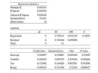
Regresslog_losagainst all variables that start with the letters_S. That is, against _Smeanbp1 _Smeanbp2 _Smeanbp3 _Smeanbp4 . gen log_los = log(los) . rc_spline meanbp number of knots = 5 value of knot 1 = 47 value of knot 2 = 66 value of knot 3 = 78 value of knot 4 = 106 value of knot 5 = 129 . regress log_los _S* Source | SS df MS Number of obs = 996 -------------+------------------------------ F( 4, 991) = 24.70 Model | 60.9019393 4 15.2254848 Prob > F = 0.0000 Residual | 610.872879 991 .616420665 R-squared = 0.0907 -------------+------------------------------ Adj R-squared = 0.0870 Total | 671.774818 995 .675150571 Root MSE = .78512 ------------------------------------------------------------------------------ log_los | Coef. Std. Err. t P>|t| [95% Conf. Interval] -------------+---------------------------------------------------------------- _Smeanbp1 | .0296009 .0059566 4.97 0.000 .017912 .0412899 _Smeanbp2 | -.3317922 .0496932 -6.68 0.000 -.4293081 -.2342762 _Smeanbp3 | 1.263893 .1942993 6.50 0.000 .8826076 1.645178 _Smeanbp4 | -1.124065 .1890722 -5.95 0.000 -1.495092 -.7530367 _cons | 1.03603 .3250107 3.19 0.001 .3982422 1.673819 ------------------------------------------------------------------------------
Test the null hypothesis that there is a linear relationship between meanbp and log_los. y_hat is the estimated expected value of log_los under this model. . predict y_hat, xb Graph a scatterplot oflog_losvs.meanbptogether with a line plot of the expectedlog_los vs. meanbp. . scatter log_los meanbp ,msymbol(Oh) /// > || line y_hat meanbp /// > , xlabel(25 (25) 175) xtick(30 (5) 170) clcolor(red) /// > clwidth(thick) xline(47 66 78 106 129, lcolor(blue)) /// > ylabel(`yloglabel', angle(0)) ytick(`ylogtick') /// > ytitle("Length of Stay (days)") /// > legend(order(1 "Observed" 2 "Expected")) name(knot5, replace) . test _Smeanbp2 _Smeanbp3 _Smeanbp4 ( 1) _Smeanbp2 = 0 ( 2) _Smeanbp3 = 0 ( 3) _Smeanbp4 = 0 F( 3, 991) = 30.09 Prob > F = 0.0000
Define 6 spline covariates associated with 7 knots at their default locations. . drop _S* y_hat . rc_spline meanbp, nknots(7) number of knots = 7 value of knot 1 = 41 value of knot 2 = 60 value of knot 3 = 69 value of knot 4 = 78 value of knot 5 = 101.3251 value of knot 6 = 113 value of knot 7 = 138.075 . regress log_los _S* { Output omitted } . predict y_hat, xb . scatter log_los meanbp ,msymbol(Oh) /// > || line y_hat meanbp /// > , xlabel(25 (25) 175) xtick(30 (5) 170) clcolor(red) /// > clwidth(thick) xline(41 60 69 78 101 113 138, lcolor(blue)) /// > ylabel(`yloglabel', angle(0)) ytick(`ylogtick') /// > ytitle("Length of Stay (days)") /// > legend(order(1 "Observed" 2 "Expected")) name(setknots, replace)
Define 6 spline covariates associated with 7 knots at evenly spaced locations. . drop _S* y_hat . rc_spline meanbp, nknots(7) knots(40(17)142) number of knots = 7 value of knot 1 = 40 value of knot 2 = 57 value of knot 3 = 74 value of knot 4 = 91 value of knot 5 = 108 value of knot 6 = 125 value of knot 7 = 142 . regress log_los _S* { Output omitted } . predict y_hat, xb . scatter log_los meanbp ,msymbol(Oh) /// > || line y_hat meanbp /// > , xlabel(25 (25) 175) xtick(30 (5) 170) clcolor(red) /// > clwidth(thick) xline(40(17)142, lcolor(blue)) /// > ylabel(`yloglabel', angle(0)) ytick(`ylogtick') /// > ytitle("Length of Stay (days)") /// > legend(order(1 "Observed" 2 "Expected")) name(setknots, replace)
Define seto be the standard error of y_hat. Define lbandubto be the lower and upper bound of a 95% confidence interval for y_hat. This twoway plot includes an rarea plot of the shaded 95% confidence interval for y_hat. . drop _S* y_hat . rc_spline meanbp, nknots(7) { Output omitted } . regress log_los _S* { Output omitted } . predict y_hat, xb . predict se, stdp . generate lb = y_hat - invttail(_N-7, 0.025)*se . generate ub = y_hat + invttail(_N-7, 0.025)*se . twoway rarea lb ub meanbp , bcolor(gs6) lwidth(none) /// > || scatter log_los meanbp ,msymbol(Oh) mcolor(blue) /// > || line y_hat meanbp, xlabel(25 (25) 175) xtick(30 (5) 170) /// > clcolor(red) clwidth(thick) ytitle("Length of Stay (days)") /// > ylabel(`yloglabel', angle(0)) ytick(`ylogtick') name(ci,replace) /// > legend(rows(1) order(2 "Observed" 3 "Expected" 1 "95% CI" ))
Define rstudentto be the studentized residual. . predict rstudent, rstudent Plot a lowess regression curve of rstudentagainst meanbp . lowess rstudent meanbp /// > , yline(-2 0 2) msymbol(Oh) rlopts(clcolor(green) clwidth(thick)) /// > xlabel(25 (25) 175) xtick(30 (5) 170)
Simple logistic regression of hospdead against meanbp . logistic hospdead meanbp Logistic regression Number of obs = 996 LR chi2(1) = 29.66 Prob > chi2 = 0.0000 Log likelihood = -545.25721 Pseudo R2 = 0.0265 ------------------------------------------------------------------------------ hospdead | Odds Ratio Std. Err. z P>|z| [95% Conf. Interval] -------------+---------------------------------------------------------------- meanbp | .9845924 .0028997 -5.27 0.000 .9789254 .9902922 ------------------------------------------------------------------------------ . predict p,p . line p meanbp, ylabel(0 (.1) 1) ytitle(Probabilty of Hospital Death)
Logistic regression of hospdead against spline covariates for meanbp with 5 knots. Spline covariates are significantly different from zero . logistic hospdead _S*, coef Logistic regression Number of obs = 996 LR chi2(4) = 122.86 Prob > chi2 = 0.0000 Log likelihood = -498.65571 Pseudo R2 = 0.1097 ------------------------------------------------------------------------------ hospdead | Coef. Std. Err. z P>|z| [95% Conf. Interval] -------------+---------------------------------------------------------------- _Smeanbp1 | -.1055538 .0203216 -5.19 0.000 -.1453834 -.0657241 _Smeanbp2 | .1598036 .1716553 0.93 0.352 -.1766345 .4962418 _Smeanbp3 | .0752005 .6737195 0.11 0.911 -1.245265 1.395666 _Smeanbp4 | -.4721096 .6546662 -0.72 0.471 -1.755232 .8110125 _cons | 5.531072 1.10928 4.99 0.000 3.356923 7.705221 ------------------------------------------------------------------------------ . drop _S* p . rc_spline meanbp number of knots = 5 value of knot 1 = 47 value of knot 2 = 66 value of knot 3 = 78 value of knot 4 = 106 value of knot 5 = 129
We reject the null hypothesis that the log odds of death is a linear function of mean BP. . test _Smeanbp2 _Smeanbp3 _Smeanbp4 ( 1) _Smeanbp2 = 0 ( 2) _Smeanbp3 = 0 ( 3) _Smeanbp4 = 0 chi2( 3) = 80.69 Prob > chi2 = 0.0000
Estimated Statistics at Given Mean BP p = probability of death logodds = log odds of death stderr = standard error of logodds (lodds_lb, lodds_ub) = 95% CI for logodds (ub_l, ub_p) = 95% CI for p . predict p,p . predict logodds, xb . predict stderr, stdp . generate lodds_lb = logodds - 1.96*stderr . generate lodds_ub = logodds + 1.96*stderr . generate ub_p = exp(lodds_ub)/(1+exp(lodds_ub)) . generate lb_p = exp(lodds_lb)/(1+exp(lodds_lb)) . by meanbp: egen rate = mean(hospdead) rate = proportion of deaths at each blood pressure . twoway rarea lb_p ub_p meanbp, bcolor(gs14)/// > || line p meanbp, clcolor(red) clwidth(medthick) /// > || scatter rate meanbp, msymbol(Oh) mcolor(blue) /// > , ylabel(0 (.1) 1, angle(0)) xlabel(20 (20) 180) /// > xtick(25 (5) 175) ytitle(Probabilty of Hospital Death) /// > legend(order(3 "Observed Mortality"/// > 2 "Expected Mortality" 1 "95% CI") rows(1))
We can use this model to calculate mortal odds ratios for patients with different baseline blood pressures. . list _S* /// > if (meanbp==60 | meanbp==90 | meanbp==120) & meanbp ~= meanbp[_n-1] +-------------------------------------------+ | _Smean~1 _Smean~2 _Smean~3 _Smean~4 | |-------------------------------------------| 178. | 60 .32674 0 0 | 575. | 90 11.82436 2.055919 .2569899 | 893. | 120 56.40007 22.30039 10.11355 | +-------------------------------------------+ Logodds of death for patients with meanbp = 60 Logodds of death for patients with meanbp = 90 . lincom (5.531072 + 60*_Smeanbp1 + .32674*_Smeanbp2 /// > + 0*_Smeanbp3 + 0 *_Smeanbp4) /// > /// > -(5.531072 + 90*_Smeanbp1 + 11.82436*_Smeanbp2 /// > + 2.055919*_Smeanbp3 + .2569899*_Smeanbp4)
Mortal odds ratio for patients with meanbp = 60 vs. meanbp = 90. . lincom (5.531072 + 120*_Smeanbp1 + 56.40007*_Smeanbp2 /// > + 22.30039*_Smeanbp3 + 10.11355*_Smeanbp4) /// > /// > -(5.531072 + 90*_Smeanbp1 + 11.82436*_Smeanbp2 /// > + 2.055919*_Smeanbp3 + .2569899*_Smeanbp4) ( 1) 30 _Smeanbp1 + 44.57571 _Smeanbp2 + 20.24447 _Smeanbp3 + 9.85656 > _Smeanbp4 = 0 ------------------------------------------------------------------------------ hospdead | Odds Ratio Std. Err. z P>|z| [95% Conf. Interval] -------------+---------------------------------------------------------------- (1) | 2.283625 .5871892 3.21 0.001 1.379606 3.780023 ------------------------------------------------------------------------------ Mortal odds ratio for patients with meanbp = 120 vs. meanbp = 90. ( 1) - 30 _Smeanbp1 - 11.49762 _Smeanbp2 - 2.055919 _Smeanbp3 - > .2569899 _Smeanbp4 = 0 ------------------------------------------------------------------------------ hospdead | Odds Ratio Std. Err. z P>|z| [95% Conf. Interval] -------------+---------------------------------------------------------------- (1) | 3.65455 1.044734 4.53 0.000 2.086887 6.399835 ------------------------------------------------------------------------------
Stata Software Goldstein, R: srd15, Restricted cubic spline functions. 1992; STB-10: 29-32. spline.ado Sasieni, P: snp7.1, Natural cubic splines. 1995; STB-24. spline.ado Dupont WD, Plummer WD: rc_spline from SSC-IDEAS http://fmwww.bc.edu/RePEc/bocode/r General Reference Harrell FE: Regression Modeling Strategies: With Applications to Linear Models, Logistic Regression, and Survival Analysis. New York: Springer, 2001. Stone CJ, Koo CY: Additive splines in statistics Proceedings of the Statistical Computing Section ASA. Washington D.C.: American Statistical Association, 1985:45-8.
Cubic B-Splines de Boor, C: A Practical Guide to Splines. New York: Springer-Verlag 1978 • Similar to restricted cubic splines • More complex • More numerically stable • Does not perform as well outside of the knots Software Newson, R: sg151, B-splines & splines parameterized by values at ref. points on x-axis. 2000; STB-57: 20-27. bspline.ado
nl – Nonlinear least-squares regression • Effective when you know the correct form of the non-linear relationship between the dependent and independent variable. • Has fewer post-estimation commands and predict options than regress.
Conclusions • Restricted cubic splines can be used with any regression program that uses a linear predictor – e.g. regress, logistic, glm, stcox etc. • Can greatly increase the power of these methods to model non-linear relationships. • Simple technique that is easy to use and easy to explain. • Can be used to test the linearity assumption of generalized linear regression models. • Allows users to take advantage of the very mature post-estimation commands associated with generalized linear regression programs to produce sophisticated graphics and residual analyses.