APPLICATIONS OF THE FIRST LAW Kinetic theory and internal energy: predicting the specific heats of dry air Application
APPLICATIONS OF THE FIRST LAW Kinetic theory and internal energy: predicting the specific heats of dry air Applications of the first law Kirchoff’s theorem Poisson’s equation Potential temperature. KINETIC THEORY AND INTERNAL ENERGY

APPLICATIONS OF THE FIRST LAW Kinetic theory and internal energy: predicting the specific heats of dry air Application
E N D
Presentation Transcript
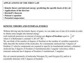
APPLICATIONS OF THE FIRST LAW • Kinetic theory and internal energy: predicting the specific heats of dry air • Applications of the first law • Kirchoff’s theorem • Poisson’s equation • Potential temperature KINETIC THEORY AND INTERNAL ENERGY Without delving into the kinetic theory of gases, we can make use of one of its results in order to obtain some insight into internal energy. each molecule possesses an amount of energy per degree of freedom equal to where k is Boltzmann’s constant=1.381023 JK-1 . We can think of the number of degrees of freedom as the number of variables required to fully describe the motion of the molecules. So a monatomic molecule has 3 degrees of freedom (3 velocity components are required to specify its translational motion), a diatomic molecule has 5 degrees of freedom (3 translational plus 2 angular velocities), while a triatomic molecule has 6 degrees of freedom (3 translational, 3 angular). Dry air consists primarily of molecular Nitrogen (N2) and Oxygen (O2) and so is essentially diatomic with 5 degrees of freedom.
Hence the internal energy per mole is given by: (4.1) where n is the number of degrees of freedom and NA is Avogadro’s number equal to NA=6.021023 mol-1 . Note: Boltzmann’s constant may therefore be thought of as the universal gas constant per molecule. The internal energy per kilogram (i.e., the specific internal energy) is therefore given by: (4.2) where M is the molecular weight of the gas. Thus, we would predict that for dry air, and since then . Moreover, since cp-cv=R, then we can also predict that for dry air . Using R=287.05 Jkg-1K-1 , our prediction becomes for dry air: cp=1005 Jkg-1K-1 . The table below shows that this prediction compares rather well with observations.
Table 4.1: Measured specific heat capacity at constant pressure, cp, for dry air.
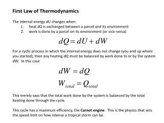
POISSON’S EQUATIONS Despite the fact that energy in the atmosphere/ocean system ultimately comes from radiative heating, adiabatic processes in the atmosphere are of interest for several reasons. Often it is because real atmospheric processes occur quickly in comparison with the time scale for heat transfer, and so may be considered to be approximately adiabatic. Alternatively, we may wish to make the adiabatic assumption simply because we are ignorant of the heat transfer and consequently must ignore it or give up. Poisson’s equations describe relationships between the state variables T, p, and for adiabatic processes. When q=0 (adiabatic process), the first version of the first law may be written: (4.5) Substituting for p from the ideal gas law, dividing by cvT, and using R=cp-cv we have, after some manipulation: (4.6) where =cp/cv (=7/5 for an ideal gas). This implies that, for an ideal gas undergoing an adiabatic process: (4.7) Eq. (4.7) is one of three Poisson equations.
Eq. (4.7) can be used to explain a number of atmospheric phenomena. For example: • When you compress the air in a bicycle pump, v decreases and hence T increases and the • air warms. (Sometimes the bicycle pump is noticeably warmer after use.) • 2. A similar explanation can be offered for the heating of subsiding (i.e., descending) air that • gives rise to a Chinook. • 3. Conversely, in a rising, expanding thermal, v increases and so T falls. This is a dynamical • component that contributes to the decrease of temperature with height in the troposphere. • (The other component is the height dependence of absorption of longwave radiation emitted by • the Earth.) Starting with the second version of the first law, Eq. (3.8) and following a similar manipulation, one may arrive at the second Poisson equation for an adiabatic process in an ideal gas: (4.8) where =R/cp (=2/7 for an ideal gas). Finally, by combining Eqs. (4.7) and (4.8), we arrive at the third Poisson equation: (4.9) Where = cp / cv=7/5. Eq. (4.9) is the most familiar of Poisson’s equations, although they are all equivalent.
POTENTIAL TEMPERATURE Meteorologists use Eq. (4.8) to define a quantity known as potential temperature (a thermodynamic concept that seems to be unique to meteorology). Suppose we start with a parcel of air in some arbitrary initial state specified by T, p. Let us move the air parcel adiabatically to a pressure of 100 kPa and call the temperature which it achieves the potential temperature, . By using Eq. (4.8) in the initial and final states, it can be easily shown that: (4.10) Where p must be express in kPa (since we have used 100 kPa in the numerator). Because the potential temperature of an air parcel is conserved under dry adiabatic processes, it may be used as a tracer for air parcels. Isentropic coordinates are ones in which potential temperature is used as the vertical coordinate instead of height. In such a coordinate system, a parcel of dry air undergoing only adiabatic processes will always remain on the same coordinate surface. [NOTES: Why they are called isentropic coordinates will become clear when we discuss entropy and the Second Law of TD. We will also take into account the presence of water vapour. A similar concept is used in oceanography. These are isopycnal coordinates.] The first law of thermodynamics may be expressed in yet a third version using potential temperature. Let us begin with the definition of potential temperature, Eq. (4.10), take logarithms and then total differentials:
(4.11) Multiplying by cp and using the ideal gas law and the second version of the first law: (4.12) This third version of the first law has several useful features. It is somewhat simpler than the previous two versions, it expresses the fact that the potential temperature is constant for adiabatic processes and varies for diabatic processes, and it seems to imply that the quantity on the right hand side is a function of state (since the potential temperature is a function of state). We will encounter q/T again soon in conjunction with the Second Law of Thermodynamics. By considering Eq. (4.12) along with the first version of the first law for a cycle, and remembering that a function of state does not change in a cyclic process (e.g., ), it is easy to show that The integral on the right hand side is the net work done during the cycle. Hence this equation implies that on a graph with axes cpln and T, the area enclosed by a cycle will equal the work done during the cycle. We will make use of this fact later when we consider the Tephigram.
THE SECOND LAW OF THERMODYNAMICS • Thermodynamic surface for an ideal gas • Second Law • Entropy THERMODYNAMIC SURFACE FOR AN IDEAL GAS The ideal gas law is the equation of a surface in a three-dimensional space whose coordinates are p, v, and T. This surface constitutes the ensemble of all states of an ideal gas that are permitted by the ideal gas law. It is called the thermodynamic surface for that gas. Any changes in the gas’ state variables simply reflects movement on this surface. The following diagram illustrates this surface and on it are examples of isobaric, isothermal, isosteric, and adiabatic processes. Such processes may all be represented in the form: (5.1) Where n=0 is an isobar, n=1 is an isotherm, n= is an adiabat, and nis an isostere. [NOTE: an isosteric process is one for which the specific volume remains constant. Such a process is also an isopycnic process because the density is constant. Processes for which the total volume of the air parcel remains constant are called isochoric.]
SECOND LAW Sometimes the use of the first law will give rise to a seemingly impossible result. How do we know that it is impossible? Because it is entirely inconsistent with our collective experience. As an example, consider the cooling of bathwater. We will assume this to be an isobaric process, so that the first law is : (5.2) Let us imagine that 100 litres of water cool from 50oC to 20oC. If that heat is given to 10 kg of air in the bathroom (assuming the bathroom to be well insulated so that no heat is lost), what will be the final temperature of the air? If the warming of the air also occurs isobarically then the first law for the air is: (5.3) Equating the Q’s in Eqs. (5.2) and (5.3), we can solve for dTausing cp=1.0103 Jkg-1K-1 and cw=4.2103 Jkg-1K-1. The temperature change of the air is 1.3103 K!!! We know this result is impossible, but it follows from the first law, so what is wrong? Clearly, in the final stages of the process as we have envisaged it, the air will be warmer than the bathwater. And yet we have implicitly assumed that heat will continue to flow from the water into the air to warm it. Experience tells us that heat simply does not flow spontaneously from a colder to a warmer body. This is called the Clausius formulation of the second law.
Rudolf Clausius (1822-1888) was a German physicist who established the foundations of modern thermodynamics in a seminal paper of 1850. He introduced the concepts of internal energy and entropy (from the Greek for transformation). His great legacy to physics was the concept of the irreversible increase of entropy (“Die Energie der Welt ist constant; die Entropie strebt einen Maximum zu.” (1865)).
A more precise expression of the Clausius formulation is: “It is impossible to construct a cyclic engine that will produce the sole effect of transferring heat from a colder to a hotter reservoir.” The term “sole effect” means that no work can be done. Of course heat pumps exist, so it is possible to transfer heat from a colder to a warmer reservoir, but only by doing work. Oxford physicist P.W. Atkins in his book entitled “The Second Law” states it in yet another way (p. 9): “…although the total quantity of energy must be conserved in any process….the distribution of that energy changes in an irreversible manner.” He also talks about a “fundamental tax,” stating that “Nature accepts the equivalence of heat and work, but demands a contribution whenever heat is converted into work.” (p. 21). Note, however, that there is no tax when work is converted into heat (for example, by friction). Since we may think of heat as disordered motion, and work as ordered motion, it would appear that the second law also has something to say about a fundamental disymmetry between order and disorder. In order to formulate the second law mathematically, we will take another look at the bathtub problem, invoking a cyclic engine to transfer the heat between the room air and the water in the tub, as in the following diagram.
We will focus our attention this time on the thermodynamics of the cyclic engine. Let us suppose that TwTa . Let qa be the heat added to the engine by the room air, and let qw be the heat added to the engine by the bath water. Our second law experience says that the former will be positive and the latter negative (that is the air, being warmer, will give up heat to the engine and the bathtub water will gain heat from the engine). Moreover, the first law requires that the magnitudes of these heat transfers must be the same. Hence we may write qa =q= -qwwhere we insist that the quantityq must be positive. Let us now consider . Why we do this is not immediately obvious, although you should recall from last lecture that q/T is a function of state. In this case:
The inequality in Eq. (5.4) holds in general for real (irreversible) processes. The equality in Eq. (5.4) will only hold as the two temperatures become equal. Heat transfer under such near-equilibrium conditions will be very slow and essentially reversible. If we define entropy, s, as follows: (5.5) then, generally (dropping the line integral): (5.6) where the inequality holds for irreversible processes and the equality for reversible processes. Clearly for adiabatic irreversible processes, the entropy must always increase, leading to the previously mentioned statement by Clausius. [NOTE: See also Stephen Hawking’s “A Brief History of Time” for a discussion of entropy and the arrow of time (Ch. 9).] For adiabatic reversible processes, entropy remains constant. Formally, we can think of entropy as a function of state whose increase gives a measure of the energy of a system which has ceased to be available for work during a given process. Note also from last lecture that ds=cpdln for reversible processes. Therefore, processes in which potential temperature is conserved are also isentropic processes.
Although it is important to be aware of the second law of thermodynamics, the field of atmospheric thermodynamics makes little use of it. We tend to assume that atmospheric processes occur reversibly. However, since our atmosphere is in actuality an enormous heat engine that transports heat from the tropics to the poles, the concepts and ideas that arise from the second law are of some use. SUMMARY OF REVERSIBLE AND IRREVERSIBLE PROCESSES: From Zemansky and Dittman, “Macroscopic Physics”: “A reversible process is one that is performed in such a way that, at the conclusion of the process, both the system and the local surroundings may be restored to their initial states, without producing any changes in the rest of the universe.” For example, imagine a weight on a pulley. Suppose that the weight is lowered by a small amount so that work is done and a transfer of heat takes place from the system to its surroundings. If the system can be restored to its original state, I.e., the weight is lifted back up and the surroundings forced to part with the heat that they had gained during the lowering, then the original process is reversible. A little thought should convince you that no real process is reversible. The abstraction of reversible processes, however, provides a clean theoretical foundation for the description of real world, irreversible processes.
What real world processes makes things irreversible? Dissipative effects, such as viscosity, friction, inelasticity, electric resistance, and magnetic hysteresis, etc. Processes for which the conditions for mechanical, thermal, or chemical equilibrium, i.e., thermodynamic equilibrium are not satisfied. In atmospheric and oceanic sciences, it is common to assume that there are no dissipative effects (particularly for flows at large spatial scales) and that motion of the atmosphere and oceans is isentropic. Viscous and frictional dissipation do, of course, occur (particularly in the atmospheric and oceanic boundary layers) but a good understanding of the dynamics can be obtained from inviscid theory.
APPLICATIONS OF THE SECOND LAW • Carnot cycle • Applications of the second law • Combined first and second law • Helmholtz and Gibbs free energies CARNOT CYCLE The Carnot cycle is an ideal heat engine cycle that offers insights into other heat engines, including the atmosphere. It is a reversible cycle, performed by an ideal gas, that consists of two isothermal processes linked by two adiabatic processes, as illustrated below: A 1 4 B D 2 C 3
Nicolas Leonard Sadi Carnot (1796-1832) led a short but interesting life. He was able to pursue his scientific research as a result of his appointment to the army general staff. He died of scarlet fever followed by cholera, and all his papers were burned after his death. Only three major scientific works survive. His work on heat engines led to the ideal heat engine and cycle that now bear his name. Interestingly, he was able to make significant scientific advances while still believing in the erroneous caloric theory of heat, in which heat is taken to be a function of state.
For each of the four processes in the Carnot cycle, we will consider the change in internal energy, the heat added to the working gas and the work done by the gas (i.e., the components of the first law). Table 1: Thermodynamics of the Carnot cycle Notes:1) q3 is negative because we consider q to be the heat added to the system. 2) The net work done in a Carnot cycle must equal the difference between the heat input and the heat exhausted. This work is also equal to the area contained within the Carnot cycle on a p-v diagram. 3) In order to show that ds=0, we must show that vB/vA=vC/vD. This can be done by comparing the Poisson equations for the two adiabatic processes.
The efficiency of the Carnot cycle is defined to be the ratio of the mechanical work done to the heat absorbed from the hot reservoir. That is: (6.1) It can be shown that this is the maximum efficiency of any cyclic engine working between the same two temperatures. This is known as Carnot’s theorem. Note that the efficiency of the Carnot cycle can only be unity (i.e., 100%) if the cold reservoir (T3) has a temperature of absolute zero. In order to increase the efficiency of an engine, one would like to minimize T3/T1. EQUIVALENCE OF HEAT AND WORK, EFFICIENCY, AND THE FIRST LAW Recall the first law: du=q- w. If we consider an engine cycle in a p-v diagram then the path taken (clockwise for a heat engine, counterclockwise for a refrigerator) may be expressed as the line integral of the first law around the cycle: Furthermore, since du is an exact differential its line integral vanishes, leaving us with: (6.2)
i.e. there is an equivalence of net heat gained/lost and net work done by/on the system. Efficiency, E, may also be considered to be the ratio of Work Out to Heat In. Consider the following idealized engine cycle: The net heat input is QH=Q12+Q23. The net heat output is QC=Q34+Q41. The net heat in is therefore Q=QH-QC and we now know that this must be the net work done, i.e., W= QH-QC . The efficiency may then be expressed in terms of the heat as: Important Note: QH and QC here are MAGNITUDES of heat, and are therefore always positive.
Example: Suppose that the working fluid is an ideal gas. From the first law we have that dU=Q- W. The incremental work done is related to pressure and volume by W=pdV. Also, the change in internal energy dU along any branch of the cycle is equal to dU=CvdT=(Cp-nR)dT. NOTE: we are not using molar values here, so Cp-Cv=nR. Branch 12: Volume constant So heat is absorbed. Branch 23: Pressure constant Since we are dealing with an ideal gas for which we can express the change in volume in terms of the change in temperature as: So the first law along this branch gives us: q=du+pdV=(cp-nR)dT+nRdT=cpdT from which we get that: So, again, heat is absorbed.
Branch 34: Volume constant So heat is rejected. Branch 41: Pressure constant So, again, heat is rejected. The efficiency of this engine, E, is therefore: Note that since we want the MAGNITUDE of QC, the signs in the numerator are such that it is a positive quantity. What would an efficiency of 100% mean in this case? Well, we can substitute in Ti=piVi/nR for i=14 and show that in order for E to equal 1 we must have that:
where we’ve cancelled out the nR’s. Now note that V3=V4, V1=V2, p1=p4, and p2=p3 to show which can only be true if p3p4 and V4V1. In other words, 100% efficiency is only possible if the cycle collapses to a single point on the p-V diagram, and no work is done! Whoever said that doing no work is inefficient??????? In class example: Efficiency of the gasoline engine.
The atmosphere as a heat engine: Our atmosphere is heated in the tropics (say Ttropics=313K) and cools at the poles (say Tpoles=233K). If we were to imagine our atmosphere as an enormous heat engine that converts net incoming heat into work (kinetic energy) then the efficiency of this engine is only 26%. In fact, the actual efficiency is much lower than this. Sandström’s theorem (see Houghton, “The Physics of Atmospheres”) states that a steady circulation in the atmosphere can be maintained only if the heat source is situated at a higher pressure than the heat sink. Some reflection on the Carnot cycle will reveal that the theorem must be valid. Because the atmosphere of the Earth is transparent to solar radiation, the requirements of the theorem are satisfied for Earth. What about Venus?
APPLICATIONS OF THE SECOND LAW • Impossible processes • Kelvin formulation of the Second Law • Combined First and Second Laws • Helmholtz and Gibbs Free Energies Impossible Processes Impossible processes are ones that violate the second law of thermodynamics, i.e., ones for which: (Recall that for adiabatic reversible processes ds=0. These processes are therefore called isentropic and have many applications to the atmosphere and oceans. Adiabatic irreversible processes have ds>0, since adiabatic processes have q=0.) 2. Kelvin Formulation of the Second Law This may be postulated as follows: “It is impossible to construct a cyclic device that will produce work and no other effect than the extraction of heat from a single heat source.” This result can be readily deduced by considering an isothermal cyclic engine in contact with a single reservoir, and examining the consequences of the second law (which will demonstrate that, in fact, heat must be lost from the engine to the reservoir, and hence that work must be done on the engine).
If it were not for the second law, as expressed by Kelvin, our energy worries would vanish. We could simply extract as much work as we needed from a very large heat source such as the oceans or the interior of the Earth. 3. Combined First and Second Laws If we combine the first law in the form: (6.2) with the second law in the form: (6.3) then the combined laws take the form: (6.4) 4. Helmholtz and Gibbs Free Energies The Helmholtz and Gibbs free energies are functions of state. i.e., they are perfect differentials. They are defined, respectively, by: (6.5)
Using them, the combined first and second laws (Eq. 6.4) may be written as: where, again, the equality hold for reversible processes and the inequality holds for irreversible processes. The Helmholtz free energy is particularly useful when considering chemical reactions that occur isothermally. You’ll note that the change of the Helmholtz energy during a reversible, isothermal process equals the work done on the system, and for a reversible, isothermal, and isochoric process the Helmholtz energy is conserved. The Gibbs free energy is particularly useful when considering phase changes, which are isothermal and isobaric (and can be conceived of as occuring reversibly). Hence during such phase changes the Gibbs free energy remains constant. The Gibbs energy can be used to uniquely determine the triple point temperature and pressure of a substance, since g must be the same for the solid, liquid, and vapour phases (2 equations, 2 unknowns (T,p)). For irreversible processes, the Gibbs free energy decreases as the substance approaches its new equilibrium. It is therefore clear that an equilibrium state is one at which the Gibbs energy is at a minimum. (6.6)
Hermann von Helmholtz (1821-1894) had become the patriarch of German science by 1885. He began his career as an army doctor. As an MD and professor of physiology, he published a massive volume of work on physiological optics and acoustics. He also invented the ophthalmoscope. At the same time he began to publish work unrelated to physiology--a paper on the hydrodynamics of vortex motion in 1858, and an analysis of the motion of violin strings in 1859, for example. In 1871, Helmholtz turned his attention full-time to physics, and made significant contributions in areas ranging from electrodynamics to thermodynamics and meteorology. Josiah Willard Gibbs (1839-1903) was a Yale graduate and professor, who turned his attention to thermodynamics in the early 1870’s. He contributed to the use of geometrical methods and thermodynamic diagrams. Perhaps his most significant contribution was to the understanding of thermodynamic equilibrium, which he viewed as a natural generalization of mechanical equilibrium, both being characterized by minimum energy. He also made a substantial contribution to statistical mechanics.