Download
1 / 69
690 likes | 855 Views
Noiseless Coding. Introduction. Noiseless Coding Compression without distortion Basic Concept Symbols with lower probabilities are represented by the binary indices with longer length Methods Huffman codes, Lempel-Ziv codes , Arithmetic codes and Golomb codes. Entropy.

E N D
Introduction • Noiseless Coding Compression without distortion • Basic Concept Symbols with lower probabilities are represented by the binary indices with longer length • Methods Huffman codes, Lempel-Ziv codes, Arithmetic codes and Golomb codes
Entropy • Consider a set of symbols S={S1,...,SN}. • The entropy of the symbols is defined as where P(Si) is the probability of Si.
Example: Consider a set of symbols {a,b,c} with P(a)=1/4, P(b)=1/4 and P(c)=1/2. The entropy of the symbols is then given by
Consider a message containing symbols in S. Define rate of a source coding technique as the average number of bits representing each symbol after compressing.
Example: Suppose the following message is desired to be compressed . a a a b c a Suppose a encoding technique uses 7 bits to represent the message. The rate of the the encoding technique therefore is 7/6. (since there are 6 symbols)
Shannon’s source coding theorem: The lowest rate for encoding a message without distortion is the entropy of the symbols in the message.
Therefore, in an optimal noiseless source encoder, the average number of bits used to represent each symbol Si is It will take larger number of bits to represent a symbol having small probability.
Because the entropy is the limit of the noiseless encoder, we usually call the noiseless encoder, the entropy encoder.
Huffman Codes • We start with a set of symbols , where each symbol is associated with a probability . • Merge two symbols having lowest probabilities to a new symbol .
Repeat the merging process until all the symbols are merged to a single symbol . • Following the merging path, we can form the Huffman codes .
Example • Consider the following three symbols : a ( with prob. 0.5 ) b ( with prob. 0.3 ) c ( with prob. 0.2 )
a b c Huffman Codes : a1 b01 c00 1 1 0 0 Merging Process
Example • Suppose the following message is desired to be compressed . a a a b c a • The results of the Huffman coding are : 1 1 1 01 00 1 • Total # of bits used to represent the message : 8 bits (Rate=8/6=4/3)
If the message is not compressed by the Huffman codes , each symbol should be represented by 2 bits . Total # of bits used to represent the message therefore is 12 bits . • We have saved 4 bits using the Huffman codes .
Discussions • It does not matter how the symbols are arranged. • It does not matter how the final code tree are labeled (with 0s and 1s). • Huffman code is not unique.
Lempel-Ziv Codes • Parse the input sequence into non-overlapping blocks of different lengths. • Construct a dictionary based on the blocks. • Use the dictionary for both encoding and decoding.
It is NOT necessary to pre-specify the probability associated with each symbol.
Dictionary Generation process • Initialize the dictionary to contain all blocks of length one. • Search for the longest block W which has appeared in the dictionary. • Encode W by its index in the dictionary. • Add W followed by the first symbol of the next block to the dictionary. • Go to Step 2.
Example • Consider the following input message a b a a b a • Initial dictionary:
encoder side a b a a b a • W = a, output 0 • Add ab to the dictionary
encoder side a b a a b a • W = b, output 1 • Add ba to the dictionary
encoder side a b a a b a • W = a, output 0 • Add aa to the dictionary
encoder side a b a a b a • W = ab, output 2 • Add aba to the dictionary
encoder side a b a a b a • W = a, output 0 • Stop
decoder side • Initial dictionary • Input 0, generate a 0 a
decoder side • Receive 1, generate b • Add ab to the dictionary 1 a b
decoder side • Receive 0, generate a • Add ba to the dictionary 0 a b a
decoder side • Receive 2, generate ab • Add aa to the dictionary 2 a b a a b
decoder side • Receive 0, generate a • Add aba to the dictionary 0 a b a a b a
Example Consider again the following message a a a b c a The initial dictionary is given by
After the encoding process, the output of the encoder is given by 0 3 1 2 0 The final dictionary is given by
decoder side • Initial dictionary • Receive 0, generate a 0 a
decoder side • Receive 3, generate ? • Decoder get stuck !!! • We need Welch correction to this problem. 3 a ?
Welch correction It turns out that this behavior can arise whenever one sees a pattern of the form xwxwx where x is a single symbol, and w is either empty or a sequence of symbols such that xw already appears in the encoder and decoder table,but xwx does not.
Welch correction In this case the encoder will send the index for xw, and add xwx to the table with a new index i. Next it will parse xwx and send the new index i. The decoder will receive the index i but will not yet have the corresponding word in the dictionary.
Welch correction Therefore, when the decoder can not find the corresponding word for an index i, the word must be xwx, where xw can be found from the last decoded symbols.
decoder side Here, the last decoded symbol is a. Therefore, x=a, and w= , Hence, xwx=aa. 3 a a a
decoder side • Receive 1, generate b • Add aab to the dictionary 1 a a a b
decoder side • Receive 2 and 0, generate c and a • Final dictionary 2 0 a a a b c a
Example Consider the following message a b a b a b a After the encoding process, the output of the encoder is given by 0 1 2 4 The final dictionary is given by
decoder side • Receive 0, 1 and 2, generate a, b and ab • current dictionary 0 1 2 a b a b
decoder side • Receive 4, generate ? • current dictionary 4 a b a b ?
Here, the last decoded symbol is ab. Therefore, x=a, and w= b, Hence, xwx=aba. 4 a b a b a b a
Discussions • Theoretically, the size of the dictionary can grow infinitely large. • In practice, the dictionary size is limited. Once the limit is reached, no more entries are added. Welch had recommended a dictionary of size 4096. This corresponds to 12 bits per index.
Discussions • The length of indices may vary. When the number of entries n in the dictionary is such that 2mn > 2m-1 then the length of indices can be m.
Discussions • Use the message as an example, the encoded indices are a a a b c a 0 3 1 2 0 00 001 000 11 010 Need 13 bits (Rate=13/6)