Download
1 / 1
10 likes | 237 Views
SELF CHARACTERIZATION OF MODELLING PARAMETERS FOR SYNTHETIC APERTURE IMAGING RADIOMETERS Eric ANTERRIEU, Serge GRATTON and Bruno PICARD CERFACS 42, avenue Gaspard Coriolis 31057 TOULOUSE cedex 01 - FRANCE.

E N D
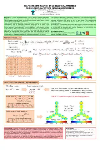
SELF CHARACTERIZATION OF MODELLING PARAMETERS FOR SYNTHETIC APERTURE IMAGING RADIOMETERS Eric ANTERRIEU, Serge GRATTON and Bruno PICARD CERFACS 42, avenue Gaspard Coriolis 31057 TOULOUSE cedex 01 - FRANCE ABSTRACT - It is now well established that Synthetic Aperture Imaging Radiometers (SAIR) promise to be powerful sensors for high-resolution observations of the Earth at low microwave frequencies. Within this context, the European Space Agency (ESA) is currently developing the SMOS space mission. Many methods have been proposed to invert the relation between the interferometric measurements and the radiometric brightness temperature of the scene under observation. It has been shown that the errors propagation through the reconstruction process depends on the regularization of the corresponding inverse problem, but also on the knowledge of the value taken by the parameters involved in the modelling of the instrument. Once the instrument is in space, these values may differ from those measured by manufacturers before launch and may also vary from one orbit to another. This is why it is necessary to have a procedure to characterize them in order to keep the errors propagation through the reconstruction process under control. This contribution describes an approach to characterize these modelling parameters, once the instrument is in orbit, from interferometric measurements over a radiometric brightness temperature field which is more or less known. The corresponding optimization problem is solved with the aid of the most up to date methods in numerical analysis. Performances of this approach are illustrated with numerical simulations showing that the value of the parameters involved in a modelling of the antennae gain patterns can be retrieved with an accuracy such that the propagation of errors through the reconstruction process is still under control. ACKNOWLEDGMENTS This work is supported by ESA, CNES, CNRS and the Région Midi-Pyrénées. INSTRUMENT MODELLING =sincos Interferometric measurements -2j(ukl+vkl) * ~ Vkl Fk(,) Fl(,) T(,) rkl(- ) e with: dd =sinsin 1-2-2 j(,) 6-parameters antenna gain pattern D(,) = Docos2ncos2 +cos2msin2 , ukl+vkl n=-0.15/log10cos3x F(,) =D(,)e fo 2 2 j(,) m=-0.15/log10cos3y o o F(,) =D(,)e with: (,) =[Lxsin+Lzx(1-cos)]cos2+[Lysin+Lzy(1-cos)]sin2 6 2 1 4 10 3 5 8 7 9 62.28 67.89 62.28 64.57 64.57 59.43 67.43 66.47 56.00 66.28 64.57 60.77 68.00 57.44 72.57 59.34 62.28 64.00 68.57 67.43 0.0 4.0 -1.0 -4.0 0.0 0.0 -1.0 -3.0 4.0 0.0 20.0 20.0 25.0 15.0 25.0 11.0 25.0 22.0 19.0 1.0 0.0 -3.0 2.0 1.0 2.0 1.0 2.0 2.8 0.5 1.0 -9.0 -16.0 -16.0 -25.0 -25.0 -30.0 -25.0 -12.0 -7.0 -6.0 2(n+1)(m+1) Do= , 10-antennae instrument n+m+1 3x 3y Lx Lzx Ly Lzy F(,) 0° 90° 0° 360° 2 +2 1 D(,) (,) 3x, 3y in ° Lx, Lzx, Ly, Lzyin mm CHARACTERIZATION OF MODELLING PARAMETERS Modelling operator Least-squares approach Non linear optimization: iterative DFP or BFGS scheme Over constrained problem: 90 interferometric measurements Over constrained problem: 60 unknown modelling parameters SMOS: 73 elements up to 5256 modelling parameters Vkl= (GT)kl+ noise min ||V-GT||2 3x, Lx, Lzx 3y, Ly, Lzy Initial guess: 3x= 65°, Lx=Lzx= 0 mm 3y= 65°, Ly=Lzy= 0 mm (for all the antennae) rms error on initial parameters: ~ F(,) -F(,) 0° 90° 0° 360° 50 iterations to reach minimum: = 0.005 = 0.5° ~ ~ ~ 3x 3x 3y 3y Lx Lx Lzx Lzx Ly Ly Lzy Lzy rms error on recovered parameters: 0.21 3.78 0.23 4.69 2.56 0.45 7.59 0.95 0.71 1.61 1.55 8.65 ~ ~ D(,) -D(,) (,) -(,) CONCLUSION - A method for retrieving modelling parameters from interferometric measurements over a given brightness temperature field has been introduced. It has been illustrated with an example showing that the antennae voltage patterns can be retrieved with an accuracy such that the propagation of errors through the inversion of the relation between the interferometric measurements and the radiometric brightness temperature of a scene under observation is still under control. Provided that the total number of modelling parameters of the instrument is less than the number of available interferometric measurements, this approach can be of course extended to any other modelling parameters (for example, those modelling the receivers band-pass filters when considering spatial decorrelation effects). REFERENCES E. ANTERRIEU, “Stabilized image reconstruction algorithm for synthetic aperture imaging radiometers”, Proc. IGARSS’02, Toronto (Canada), pp. 1642-1644, 2002. E. ANTERRIEU, P. WALDTEUFEL and G. CAUDAL, “About the effects of instrument errors in interferometric radiometry”, Radio Science, 38(3), 2003.