Download
1 / 54
540 likes | 672 Views
Efficiently Supporting Changes to Declarative Schema Mappings. Todd J. Green University of California, Davis. January 28, 2011 @Stanford InfoSeminar. Change is a Constant in Data Management. Databases are highly dynamic ; many kinds of changes need to be propagated efficiently:

E N D
Efficiently Supporting Changes to Declarative Schema Mappings Todd J. Green University of California, Davis January 28, 2011 @Stanford InfoSeminar
Change is a Constant in Data Management • Databases are highly dynamic; many kinds of changes need to be propagated efficiently: • To data (“view maintenance”) • To viewdefinitions (“view adaptation”) • Others, such as schema evolution, etc. • Data exchange and collaborative data sharing systems (e.g., Orchestra [Ives+ 05]) exacerbate this need: • Large numbers of materialized views • Frequent updates to data, schemas, mapping/view definitions
Change Propagation: a Problem of Computing Differences View maintenance view definition source data materialized view Given: R V change to source data (difference wrt current version) Goal: compute change to materialized view (difference) R¢ V¢ View adaptation view definition source data materialized view Given: R V Goal: change to view definition (another kind of difference) compute change to materialized view V¢
Challenges in Change Propagation • View maintenance: studied since at least the mid-eighties [Blakeley+ 86], but existing solutions quite narrow and limited • Various known methods to compute changes “incrementally”, e.g., count algorithm[Gupta+ 93] • How do we optimize this process? What is space of all update plans? • View adaptation: less attention, but renewed importance in context of data exchange/collaborative data sharing systems • Previous approaches: limited to case-based methods for simple changes [Gupta+ 01] • Complex changes? Again, space of all update plans? • Key challenge: compute changes using database queries!
Roadmap • Part I: a grand unified theory of change propagation • Part II: a practical implementation in Orchestra
Part I: Theoretical Underpinnings [Green,Ives,Tannen 09] • A novel, unified approach to view maintenance, view adaptation that allows the incorporation of optimizationstrategies: • Representing changes and data together: Z-relations • View maintenance, view adaptation as special cases of a more general problem:rewriting queries using views (on Z-relations) • A sound and complete algorithm for rewriting relational algebra (RA) queries (with difference!) using RA views on Z-relations • Enabled by the surprising decidability of Z-equivalence of RA queries • Maintaining/adapting views under bag or set semantics via excursion through Z-semantics
Representing Changes as Data: Z-Relations • Z-relation: a relation where each tuple is associated with a (positive or negative) count • Positive counts indicate (multiple) insertions; negative counts, (multiple) deletions • Uniform representation for both data and changes to data • Update application = union (a query!) • Can think of changes to data as a kind of annotated relation R¢ R’ = R [ R¢
Relational Algebra (RA) on Z-Relations join (⋈) multiplies counts union ([), projection (¼) add counts selection (¾) multiplies counts by 0 or 1 difference (–) subtracts counts Note,DifNote, difference can lead to negative counts (unlike “proper subtraction” in bag semantics where negative counts are truncated to 0) (same as for semiring-annotated relations [Green+07])
Incremental View Maintenance: An Application of Z-Relations Materialized view (with duplicates): Source relation: V(x,y) :– R(x,z), R(z,y) R 2 copies of (b,b) deletion R¢ V¢ delete 1 copy of (b,b) insertion insert 1 copy of (b,d) Delta rules[Gupta+ 93]for V with Z-relations semantics: V¢(x,y) :– R(x,z), R¢(z,y) V¢(x,y) :– R¢(x,z), R’(z,y)
Delta Rules: a Special Case ofRewriting Queries Using Views on Z-Relations Materialized views: Query (to compute diff.): V(x,y) :– R(x,z), R(z,y) R’(x,y) :– R(x,y) R’(x,y) :– R¢(x,y) V¢(x,y) :– R’(x,z), R’(z,y) – V¢(x,y) :– R(x,z), R(z,y) rewrite V¢ using the materialized views ... OTHER PLANS...? Another delta rules rewriting: Delta rules rewriting: V¢(x,y) :– R(x,z), R¢(z,y) V¢(x,y) :– R¢(x,z), R’(z,y) V¢(x,y) :– R¢(x,z), R(z,y) V¢(x,y) :– R’(x,z), R¢(z,y)
View Adaptation: Another Application of Rewriting Queries Using Views Old view definition: New view definition: V(x,y) :– R(x,z), R(z,y) V(x,y) :– R(x,z), R(y,z) V’(x,y) :– R(x,z), R(z,y) reformulate using materialized view V ... AGAIN, OTHER PLANS...? A plan to “adapt” V into V’: V’(x,y) :– V(x,y) – V’(x,y) :– R(x,z), R(y,z)
Bag Semantics, Set Semantics via Z-Semantics • Even if we can solve the problems for Z-relations, what does this tell us about the answers we actually need: for bag semantics or set semantics? • For positiveRA (RA+) queries/views on bags • Z-semantics and bag semantics agree • Further, eliminate duplicates to get set semantics • Still works if rewriting is actually in RA (introduces difference)! • Also works for RA queries/views with restricted use of difference • Still covers, e.g., the incremental view maintenance case
Z-Equivalence Coincides with Bag-Equivalence for Positive RA (RA+) Lemma. For RA+ queries Q, Q’ we have Q´Z Q’ (equivalent on Z-relations) iffQ´N Q’ (equivalent on bag relations) Corollary. Checking Z-equivalenceforRA+: convert to unions of conjunctive queries (UCQs), check if isomorphic • CQsQ´N Q’ iffQ≅Q’ [Lovász 67, Chaudhuri&Vardi 93] • UCQsQ´N Q’ iffQ≅Q’ [Cohen+ 99] Complexity of above: graph-isomorphism complete for UCQs; for RA+ (exponentially more concise than UCQs), don’t know!
Z-Equivalence is Decidable for RA Key idea. Every RA query Q can be (effectively) rewritten as a single difference A – B where A and B are positive • Not true under set or bag semantics! Corollary. Z-equivalence of RA queries is decidable Proof. A – B´ZC – D where A, B, C, D are positive ,A[D´ZB [C , A[D´NB [C which is decidable [Cohen+ 99] • Same problem undecidable for set, bag semantics! Alternative representation of relational algebra queries justified by above: differences of UCQs
Rewriting Queries Using Views with Z-Relations Given: query Q and set V of materialized views, expressed as differences of UCQs Goal: enumerate allZ-equivalent rewritings of Q (w.r.t. V) Approach: term rewrite system with two rewrite rules By repeatedly applying rewrite rules – both forwards and backwards (folding and augmentation) – we reach all (and only) Z-equivalent rewritings
An Infinite Space of Rewritings • There are only finitely many positive (nontrivial) rewritings of RA query Q using RA views V • With difference, can always rewrite ad infinitum by adding terms that “cancel” • But even without this: Now consider Q = R2 ´Z VR – R4(equiv. is w.r.t. V) ´Z VR – VR3[ R6 ´Z VR – VR3[ VR5– R8 ´Z ... Let RS denote relational composition of R with S, i.e., RS(x,y) :– R(x,z), S(z,y) Let V contain single view V = R[ R3 none of these have “cancelling” terms! repeated relational composition
How Do We Bound the Space of Rewritings? Use Cost Models! Can make some reasonable cost model assumptions: • cost(A[ B) ≥ cost(A) + cost(B) • cost(A⋈B) ≥ cost(A) + cost(B) + card(A⋈B) • etc. Theorem. Under above assumptions, can find minimal-cost reformulation of RA query Q using RA views V in a bounded number of steps
Highlights of Other Results • Z-equivalence remains decidable for RA with built-in predicates (<, ≤, >, ≥, ≠) over dense linear order • Basic idea: can linearize(cf., e.g., [Cohen+ 99])queries, then test for isomorphism e.g., Q(x,y) :- R(x,y), x ≠ yQ(x,y) :- R(x,y), x < yQ(x,y) :- R(x,y), y < x • Full characterization of class of RA queries where Z-semantics and bag semantics agree on all bag instances, hence where Z-semantics can be used for evaluation • Bad news: undecidable class • Good news: covers incremental maintenance of positive views (where difference is used only for changes to sources)
Roadmap • Part I: a grand unified theory of change propagation • Part II: a practical implementation in Orchestra
Background: Orchestra CDSS [Ives+08]a Collaborative Data Sharing System • Set of peers (e.g., collaborating life scientists), each with database, agree to share information • Peers linked via network of compositional schema mappings • define how data/updates applied to one peer instance should be transformed and applied to other peer instances • System tracks provenance (lineage) information [Green+ 07] as updates are mapped/transformed • Basis of provenance-based trust policies • Also used to guide update propagation
Example: Sharing Morphological Data Alice’s field observations: A Carol wants to gather information from Alice, Bob, uBio, and put into own data repository: Bob’s field observations: B, C Carol’s Guide to Primate Hand Colors schema mappings Can do this using schemamappings Standard species names: D
Example: Sharing Morphological Data (2) Alice’s field observations: A Datalog mappings relating databases E(name, color) :– B(id, “hand color”, color), C(id, species,_), D(species, name) E(name, color) :– A(id, species,_, “hand color”, color), D(species, name) Bob’s field observations: B, C Carol’s Guide to Primate Hand Colors: E Standard species names: D
Example: Sharing Morphological Data (2) Alice’s field observations: A Datalog mappings relating databases E(name, color) :– B(id, “hand color”, color), C(id, species,_), D(species, name) E(name, color) :– A(id, species,_, “hand color”, color), D(species, name) Bob’s field observations: B, C Carol’s Guide to Primate Hand Colors: E join Standard species names: D
Example: Sharing Morphological Data (2) Alice’s field observations: A Datalog mappings relating databases E(name, color) :– B(id, “hand color”, color), C(id, species,_), D(species, name) E(name, color) :– A(id, species,_, “hand color”, color), D(species, name) Bob’s field observations: B, C Carol’s Guide to Primate Hand Colors: E join Standard species names: D
Mapping Evolution in Orchestra [m1] gene(E,N) :- bioentry(E,T,N), term(T,"gene"). [m2] mousegene(G,N) :- gene(G,N), hasGene(G,12).
Mapping Evolution in Orchestra [m1] gene(E,N) :- bioentry(E,T,N), term(T,"gene"). [m2] mousegene(G,N) :- gene(G,N), hasGene(G,12). [m2’] mousegene(G,N) :- gene(G,N), hasGene(G,M), orgname(M,"mus musculus"). [m3] gene(E,N) :- bioentry(E,T,N), term(S,"gene"), termsyn(T,S).
Challenges in Mapping Evolution (Part II) • Can we handle changes to mappings efficiently and incrementally, and in a principled way? • Mappings in practice are very hard to get right, frequent changes/iterations required over time • Relationships among peers are clarified, new data sources become available, schemas evolve, ... • Problem is wide open! • Can we handle changes to dataand mappings at the same time? • Is there a potential performance benefit? • Can we handle/exploit provenance? • Can we do all this in a cost-based way? • Sometimes many incremental plans possible, yet the best plan might be to recompute from scratch!
Supporting Evolution in Orchestra[Green&Ives 11] • A practical, cost-based reformulationengineto propagate both kinds of changes in this context, based on methods from Part I • key: cost-based search strategies and heuristicsto prune the search space; Z-semantics and differential query plans • core of engine doesn’t even know whether it’s dealing with data updates or mapping updates or both; they all look the same • Extension of these methods to exploit provenanceinformation as used in Orchestra • Prototype implementation and experimental evaluation
Architectural Overview Basic idea: pair reformulation algorithm from Part I with DBMS cost estimator, cost-based search strategies heuristics, search strategies EFFICIENT UPDATE PLAN Changes to data, view definitions ORCHESTRA Reformulation Engine execute! (Z-semantics) plans costs V V’ DBMS Cost Estimator DBMS statistics, indices, etc old views updated views
Basic Search Strategy • Huge search space, need to prune whenever possible • Start with views fully unfolded and cancelled • Then do time-boxedhill climbing with folding/augmentation; main data structure the search heap • Parameters: • time t to allow for search, # k of one-step rewritings to add at each step, max size h of search heap, ... • while (search heap non-empty, time remains) { • 1. remove cheapest plan P from heap • 2. enumerate one-step rewritings P1, ..., Pn of P and compute their costs C1, ..., Cn • 3. pick cheapest k and add to heap }
Engineering Insights • Use quick and dirty cost estimation • using custom estimator instead of DBMS estimator improved performance ~5x • Use hash consing • testing equivalence (isomorphism) of rules is extremely common operation, needs to be very fast • using hash consing improved performance another ~5x • Use a non-imperative language • we used Java; implementation was PAINFUL • would probably have been at least as fast and 10x fewer lines of code in Prolog
Speedup is >= 30% on Typical Workloads(Warning: Unofficial Results) Composite synthetic workload, PostgreSQL 9.0, collection of 24 mappings, all randomly changed, ~10GB source database (details in paper)
Another Source of Optimization Opportunities: CDSS Provenance [Green+ 07] • Basic idea: annotate source tuples with tuple ids, combine and propagate during query processing • Abstract “+” records alternative use of data (union, projection) • Abstract “¢” records joint use of data (join) • Yields space of annotations K • K-relation: a relation whose tuples are annotated with elements from K
Combining Annotations in Queries source tuples annotated with tuple ids from K
Combining Annotations in Queries Datalog mappings E(name, color) :– B(id, “hand color”, color), C(id, species,_), D(species, name) r join r¢s¢u s u Operation x¢y means joint useof data annotated by x and data annotated by y
Combining Annotations in Queries Datalog mappings E(name, color) :– B(id, “hand color”, color), C(id, species,_), D(species, name) p q E(name, color) :– A(id, species,_, “hand color”, color), D(species, name) p¢u p¢u q¢u u Operation x¢y means joint useof data annotated by x and data annotated by y
Combining Annotations in Queries Datalog mappings E(name, color) :– B(id, “hand color”, color), C(id, species,_), D(species, name) E(name, color) :– A(id, species,_, “hand color”, color), D(species, name) p¢u + q¢u p¢u q¢u Operation x+y means alternate use of data annotated by x and data annotated by y
What Properties Do K-Relations Need? • DBMS query optimizers choose from among many plans, assuming certain identities: • union is associative, commutative • join associative, commutative, distributive over union • projections and selections commute with each other and with union and join (when applicable) • Equivalent queries should produce same provenance! Proposition. Above identities hold for queries on K-relations iff (K, +, ¢, 0, 1) is a commutative semiring
What is a Commutative Semiring? • An algebraic structure (K, +, ¢, 0, 1) where: • K is the domain • + is associative, commutative with 0 identity • ¢ is associative, commutative with 1 identity • ¢ is distributive over + • 8a2K, a¢ 0 = 0 ¢a = 0 (unlike ring, no requirement for additive inverses) • Big benefit of semiring-based framework: one framework unifies many database semantics
Semirings Explain Relationship Among Commonly-Used Database Semantics Standard database models: Ranked or uncertain data: Data access:
Semirings Unify Existing Provenance Models X a set of indeterminates, can be thought of as tuple ids Orchestra provenance model: Other models:
A Hierarchy of Provenance [Green 09] Example: 2p2r + pr + 5r2 + s most informative Orchestra’s provenance polynomials N[X] drop coefficients p2r + pr + r2 + s drop exponents 3pr + 5r + s Trio(X) B[X] drop both exp. and coeff. pr + r + s Why(X) apply absorption (pr + r´r) r + s collapse terms prs Lin(X) PosBool(X) result 0? true least informative B A path downward from K1 to K2 indicates that there exists a surjective semiring homomorphismh : K1K2
Another View of CDSS Provenance: as Graph Datalog mappings: m1: E(name, color) :– A(id, species, “hand color”, color), D(species, name) p q ¢ pq + pu u ¢ Provenance table for m1: = A.Species = D.Comm. Name = A.Character pq pu Compress table using mapping’s correspondences Rewrite mappings to fill provenance table (from Alice, Bob, uBio), and Carol’s DB (from provenance table)
Computing the Graph is Easy: Use Datalog! To record provenance for mapping m1 we convert it to pair of mappings The first rule builds the provenance table for m1. The second rule projects over m1 to populate E. E(name, color) :– A(id, species, “hand color”, color), D(species, name) M1(id, species, name, color) :– A(id, species, “hand color”, color), D(species, name) E(name, color) :- M1(id, species, color, name)
Why is Provenance Useful When Mappings Change? Example (WITHOUT provenance): E(name, color) :– A(id, species, “hand color”, color), D(species, name) E(name, color) :– C(name, color, range), G(range) 2-way join + 3-way join E’(name, color) :– A(id, species, “hand color”, color), D(species, name) E’(name, color) :– C(name, color, range), G(range) E’(name, color) :– C(name, color1, range), F(color1, color), G(range) Incremental plan to compute E’ (faster???) 2-way join + 3-way join... E’(name, color) :– E(name, color) E’(name, color) :– C(name, color1, range), F(color1, color), G(range) –E’(name, color) :– C(name, color, range), G(range)
Why is Provenance Useful When Mappings Change? (2) Example (WITH provenance): M1(name, color,...) :– A(id, species, “hand color”, color), D(species, name) M2(name, color,...) :– C(name, color, range), G(range) E(name, color) :– M1(name, color,...) E(name, color):– M2(name, color,...) 2-way join + 3-way join M1’(name, color,...) :– A(id, species, “hand color”, color), D(species, name) M2’(name, color,...) :– C(name, color1, range), F(color1, color), G(range) E’(name, color) :– M1(name, color,...) E’(name, color):– M2(name, color,...) Incremental plan to compute E’ (and mapping tables) just a 2-way join! M1’(name, color,...) :– M1(name, color,...) M2’(name, color,...) :– M2(name, color1,...), F(color1, color) E’(name, color) :– M1(name, color,...) E’(name, color):– M2(name, color,...)
Speedup with Provenance is >= 70%(but you pay for storage space) Composite synthetic workload, PostgreSQL 9.0, collection of 24 mappings, all randomly changed, ~5GB source database (details in paper)
Summary (Part II) • Optimized change propagation is feasible, and can yield large speedups • For systems like Orchestra that store provenance information, even more opportunities for optimization
Summary • Change propagation for RA views can be optimized, via rewriting queries using views and Z-relations • Sound and complete rewriting algorithm • Changes to view/mapping definitions and changes to data can be handled in the same way, via optimizing queries using materialized views • Engine doesn’t even know which kind of change it’s dealing with! • These methods can be made practical --- using cost-based, heuristic optimization --- and can yield big speedups • For systems like Orchestra that store provenance information, even more speedups are possible
NEW!!! Supported by NSF CAREER IIS- 1055107 pushing these ideas to the limit... select l_returnflag, sum(l_quantity) from lineitem where l_shipdate <= ... group by l_retur... select avg(l_quant from lineitem, orders where l_shipdate <= ... group by l_retur... select ... from ... where ... group by ... having ... Scrapple!