Implicit Methods for ODEs in Numerical Simulation
Explore the advantages of implicit integration, back Euler method, and Verlet algorithm in solving ODEs for dynamic systems. Learn how to handle stiff ODEs, convert second-order to first-order, and optimize code for efficient simulations.

Implicit Methods for ODEs in Numerical Simulation
E N D
Presentation Transcript
Implicit Methods Patrick Quirk February 10, 2005
Introduction, Motivation • Explicit methods have a difficult time with some types of ODE’s • They guess where the function is heading • Stiff ODE’s • One component big for a short time • Does not contribute later • Must make time step small for explicit to handle it
Solution – Implicit Methods • Backward Euler Method • Evaluates ƒ at the point we’re aiming at • Less guessing, more accuracy • Consequently, the step size can be larger
Implicit Methods • Last example was simplisitc • Typically cannot directly solve for yn+1 • Unless ƒ is linear • So…approximate ƒ with its Taylor Expansion
Implicit Methods • More equation manipulations are done • Allows us to approximate Δx • Albeit with an inverse of a matrix! • In general this extra computation isn’t bad • Larger time step offsets this
An Aside - Explicit Method • Verlet Algorithm • Does away with the velocity term • Stores only current, previous position • Approximates velocity by xn-xn-1
An Aside - Explicit Method • But it’s explicit! • It’s a second-order method, higher accuracy • Has the computational cost of a first-order • No numerical drift like in some other explicit and implicit methods • Easy to code! • Widely used in games and physics • Often chosen over implicit methods for these reasons
Big Picture - Implicit Methods • Explicit Method code is easy • Implicit Method code is harder • Try to make problem un-stiff if possible • Then use an explicit method and small Δt • Otherwise write an implicit solver • Use the larger time step to your advantage
Second Order ODEs • Dynamics problems are often second order • Need to convert it to a first order problem
Second Order ODEs • Introduce new variables to get first order • But this gives a 2nx2n linear system • Bad news for BEM, has to solve that system • Can we reduce the size?
Second Order ODEs • Can reduce it to nxn • Introduce some more new variables • Taylor Expand ƒ (in two dimensions) • Put that back into the equation
Second Order ODEs • Substitute the first row into the second • Regroup terms and solve for Δv • If there is a variance in time, an extra term:
Sources • SIGGRAPH Course Notes • http://www.pixar.com/companyinfo/research/pbm2001/notesd.pdf • Mathworld References • http://mathworld.wolfram.com • “A Practical Dynamics System”. Kačić-Alesić, Nordenstam, Bullock. Eurographics/SIGGRAPH 2003. • http://portal.acm.org/citation.cfm?id=846276.846278 • “Advanced Character Physics”. Thomas Jakobsen. Gamasutra. 2003 • http://www.gamasutra.com/resource_guide/20030121/jacobson_01.shtml
Interactive Animation of Structured Deformable Objects Mathieu Desbrun, Peter Schröder, Alan Barr Caltech
Introduction, Motivation • Interactive deformation is tough • Simulation methods are too slow • Usually used in VR, user has control • Limited greatly by time step • Too big means instability in simulation • Too small means alteration in reality • Implicit Integration • Offers low computational time • Nearly arbitrary time step
Implicit Integration : 1D case • Replace all forces at time t by t+1 • Now positions are not blindly reached, but are logically inferred. n+1 • In other words: • Explicit steps into the unknown with only initial conditions. • Implicit tries to hit the next position correctly.
Implicit Integration : 1D case • Must compute Fn+1 at t+dt (spring forces) • Use a first order approximation (since we don’t know what exactly Fn+1(t+dt) is) • Here Δn+1x is called the backward difference operator:
Implicit Integration : 1D case • Add artificial viscosity • Increases stability • Force filtering • Uses matrix multiplication (H=dF/dx) • Global force effects • Smoothes large force differences • Pull it all together…
Implicit Integration : 1D case • Final Form for 1D: • Look closely, is it really implicit? Damping Force Force Filter Matrix
Loss in accuracy Force smoothing Artificial viscosity Force filtering matrix changes at each time step (2D/3D only) Forces you to solve a linear system Gain in speed Gain in speed Gain in speed Implicit Integration : 1D case Bad Good
Some of the “Bads” aren’t all that bad: Artificial viscosity It is frequently added to simulations. If it is already taken care of, so much the better. Changing filter matrix Even if this does take time, the computational advantages are already so significant it doesn’t matter too much. Approximating it makes it a constant Compute it once, use it forever Implicit Integration: 1D case
Similar to 1D case, though the smoothing matrix changes with each step. This paper removes the need to solve a linear system Splits the force into a linear and non-linear part Linear is easily solved, non-linear approximated to zero Magnitude does not change (internal forces), just direction Preserve linear/angular momenta Includes inverse dynamics to remove stretching Implicit Integration: 2D/3D case
Implicit Integration : 2D/3D case • In 2D/3D, implicit integration is done by computing the Hessian matrix H • It depends on position of particle nodes, changing • Equation for one element of H is too long to show here • Each node is a 3x3 matrix, total of 3nx3n elements • Too large to solve efficiently • Approximate it
Implicit Integration : 2D/3D case • Matrix split into 2 parts • Linear • Non-Linear • Simple, assume its zero • It’s constant in magnitude, but will rotate
Implicit Integration : 2D/3D case • Check if linear, angular momenta are conserved • Linear is • Sum of artificial viscosity forces is zero • Force filtering has no effect • Angular is not! • Because of that assumption about the non-linear hessian • Desbrun corrects this with some inverse dynamics
Sources • “Interactive Animation of Structured Deformable Objects”. Desbrun, Schröder, Barr. Graphics Interface. 1999 • http://www.multires.caltech.edu/pubs/GI99.pdf