Download

1 / 15
150 likes | 238 Views
Explore the N-S model in global sourcing, focusing on ownership structures, location choices, variable and fixed costs, and equilibrium decisions for firms with varying productivity levels. Analyze the effects of heterogeneity within sectors and industry variations on organizational prevalence.

E N D
Global Sourcing Antras & Helpman 2004
Overview • N-S Model • Final Goods Producers situated in North. • Choice oflocationtosourceinputs • Equilibrium in which firms with different productivity levels choose different ownership structures • Effects of within-sectoral heterogeneity and variations in industry on prevalance of organizational forms. • Antràs 2003 with incorporation of heterogeneity a la Melitz 2003.
Background • Different ownership models: Standard vertical integration, FDI, outsourcing abroad, outsourcing in domestic country • Example: Intel’s FDI strategy • Example: Nike’s arm’s-length import strategy • Powerful role of international specialization • WTO 1998 Annual Report: In the production of an American car, 30% of the car’s value in Korea, 17.5%in Japan, 7.5% in Germany…only 37% of production value in America!
The Model • representative consumer in each country with quasi-linear preferences: • Aggregate consumption in sector j is a CES function • Elasticity of substitution within sector between varieties: 1/1-Alpha • Inverse Demand function:
Technology • Producers of differentiated goods face a perfectly elastic supply of labor. • wN > wS • Monopolistic competition • As in Melitz (2003), producers needs to incur sunk entry costs wN fE, after which they learn their productivity: θ ∼ G (θ). • As in Antràs (2003a), final-good production combines two specialized inputs, according to the technology:
Technology • H: final-good producer (agent H), m: supplier (agent M). • Sectors vary in their intensity of headquarter services • Within sectors, firms differ in productivity θ • After observing θ, H decides exit or produce. • Producing incurs additional fixed costs depending on • k ∈ {V, O} and l ∈ {N, S},
Contracts • Incomplete contracts: • δN ≥ δS In times of contractual breach, Integration in North can recover a higher fraction of output. • The outside option of H under outsourcing is zero. • The outside option of M is zero regardless of ownership structure and location. • H’s profit-maximizing organizational mode will also maximize joint profits.
Equilibrium • Profit function: • By choosing k and l, H is chooses triplet (βlk, wl, f lk) • Profit is decreasing in f and w • πlk is largest when βlk = β∗(η)
Industry Equilibrium • Upon observing θ, a final-good producer H chooses the ownership structure and the location maximizing profit, or exits the industry and forfeits the fixed cost of entry wN fE • j • Firms with θ ≥ θ (X) stay in the industry • Free entry condition:
Organizational Forms: Trade offs • Location decision: Variable costs are lower in the South, but fixed costs are higher there. • Integration decision: Integration improves efficiency of variable production when the intensity of headquarter services is high, but involves higher fixed costs. This decision will depend on η, but also on θ.
Component Intensive Sector • This implies ψO (η) > ψV (η) for l = N, S, which together with the fixed costs ordering implies that any form of integration is dominated in equilibrium.
Headquarter Intensive Sector • All four organizational forms exist in equilibrium
Relative Prevalence • Relative prevalence is measured by the share of products produced in various organizational forms (V or O, in N or S). • Distribution: • σMO: the fraction of active firms that outsource in country l in the component-intensive sector. • Then: • Substituting for the cutoffs yields:
Relative Prevalance – Component-intensive • Decline in Southern wage rate? • Fall in Transport costs? • Increase in dispersion of productivity? z
Relative Prevalance – Headquarter-intensive • A fall in the relative wage in the South or in trading costs, raise the share of imported inputs and also raise outsourcing relative to integration in every country. • Industries with more productivity dispersion (lower z), have a higher share of imported inputs and integration is higher relative to outsourcing in every country. • Sectors with higher headquarter intensity (higher η), the share of imported inputs is lower and integration is higher relative to outsourcing. Consistent with Antràs (2003a) that the share of intra-firm imports in total U.S. imports is significantly higher, the higher the R&D intensity of the industry.