Download
1 / 17
170 likes | 304 Views
Modeling Crypto Occurrence, Using Lab-Specific Matrix Spike Recovery Data. Michael Messner , Ph.D. Mathematical Statistician EPA Office of Ground Water and Drinking Water Standards and Risk Management Division Messner.Michael@epa.gov. Outline. Disclaimer Data Used

E N D
Modeling Crypto Occurrence, Using Lab-Specific Matrix Spike Recovery Data Michael Messner, Ph.D. Mathematical Statistician EPA Office of Ground Water and Drinking Water Standards and Risk Management Division Messner.Michael@epa.gov
Outline • Disclaimer • Data Used • Uncertainty in Crypto Numbers Spiked • Model Building • Preferred Model (Model 5) • Results of Recovery Modeling • Informing the Crypto Occurrence Model
Disclaimer • Views expressed in this presentation are the authors and are not necessarily those of the USEPA.
Data Used • Results were obtained from analyses of 1263 source water samples that were spiked with Cryptosporidium (matrix spike samples). • Dates range from Feb, 2004 to May 2008. • For each matrix spike sample, the data include: • Organization (Lab ID) • Sample volume filtered • Sample volume spiked • Number of Crypto measured • Number of Crypto spiked • The fraction of volume spiked is found by dividing “Sample volume filtered” by “Sample volume spiked”
Uncertainty in Crypto Numbers Spiked • Spiking suspensions (“tubes”), provided by two vendors, were prepared using flow cytometry. • Both vendors checked hundreds of their tubes by carefully counting the tubes’ oocysts. • Based on data provided by one lab, a pooled estimate of relative standard deviation (RSD) is 1.35%. • The other lab provided a histogram, rather than statistical summaries. The next slide shows that their precision appears to match that of the first lab.
Histogram of Lab 2and Normal Density Function mu = 100, s = 1.35
Model Building • All models assume that the number of oocysts counted is Binomial with parameters N (exact number of oocysts in the spiked sample) and r, the probability that an oocyst in the sample will be observed and counted. • All the models account for uncertainty in N, based on 1.35% RSD. • Basic modeling approach was to start simple, using 2-parameter models, using log likelihood to gauge model quality.
Models • Model 1: r varies from assay to assay (both within and between labs) as a beta random variable. • Model 2: ln(r/(1-r)) = logit(r) varies from assay to assay as a normal random variable. • Model 3: With probability z, r varies as a Beta random variable, but the rest of the time (1-z), r is exactly zero. • Model 4: With probability z, logit(r) varies as a normal random variable, but the rest of the time (1-z), r is exactly zero. • Model 5: Both the probability of zero recovery and expected value of logit(r) vary from lab to lab as a bivariate normal random variable. Covariance allows these two features to be related.
Model 5 Hierarchy • High Level: • Grand means (mu0 and mu1) of lab-specific parameters logit(r) & pr{r=0} • Precision matrix R (R-1 = var-covar matrix) • Within-lab precision parameter phi0 • Medium Level: • Lab-specific averages of logit(r) • Lab-specific pr{r=0} • Low Level: • Sample-specific recoveries (product of nonzero recovery and an indicator of zero recovery • Data (not shown in the figure). • K ~ dbinom(N,r) • Number spiked (Sp) • Number counted (K)
Results • WinBUGS generates statistics about the model parameters and a Markov Chain Monte Carlo (MCMC) or “uncertainty” sample. • MCMC sample of size 10K takes about 4 min.
Results 0 not in interval for logit(r) and logit(z) reject hypothesis that median probabilities for these are 0.5. 0 in interval covariance is not significant, so can’t reject notion that Pr{zero} is distributed independently of median recovery (when not zero) Can’t say that Labs with poor recovery don’t also have high probability of totally missing spiked oocysts.
Labs Differ w.r.t. Mean Logit(r) Central Value Posterior median for this lab is -1.019 median r = 26.5% Average Recovery* = 24.2% Logit(0.881) = 2 Logit(0.731) = 1 Logit(0.5) = 0 Logit(0.269) = -1 Logit(0.119) = -2 Posterior median for this lab is 0.2353 median r = 55.9% Average Recovery* = 62.4% Posterior median for this lab is - 0.5883 median r = 64.3% Average Recovery* = 65.3% * (count/expected), averaged across samples
Labs Differ w.r.t. Pr{r=0} Lab found Crypto in all 60 spikes Lab found no Crypto in 5 of 76 spikes Lab found no Crypto in 17 of 223 spikes Lab found no Crypto in 4 of 22 spikes
Informing the Occurrence Model • Okay, so what good is all this? • Can use MCMC sample to inform our upcoming estimate of the Long-Term Rule’s (LT2’s) benefit. • Public water systems are monitoring their source waters for Crypto. • The new Crypto data, together with a model that accounts for lab-specific recovery will produce better estimates of actual occurrence. • Better occurrence estimates better risk analyses improved estimate of the benefit of treatment changes that result from LT2 implementation.
The funny thing about hierarchical models… …is that, once you’ve tried one (and succeeded), you’ll see hierarchical models everywhere… …which makes you wonder if you’re like that fellow with a hammer, to whom every problem looks like a nail. Hierarchical modeling : Try it, you’ll like it.