Download
1 / 12
120 likes | 209 Views
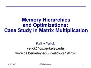
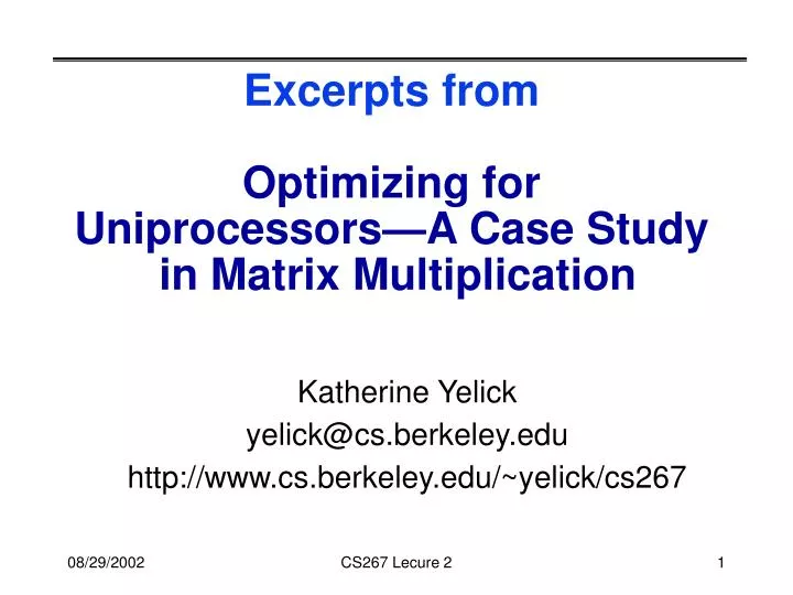
Excerpts from Optimizing for Uniprocessors—A Case Study in Matrix Multiplication. Katherine Yelick yelick@cs.berkeley.edu http://www.cs.berkeley.edu/~yelick/cs267. Computational Intensity: Key to algorithm efficiency. Key to machine efficiency.

E N D
Excerpts from Optimizing for Uniprocessors—A Case Study in Matrix Multiplication Katherine Yelick yelick@cs.berkeley.edu http://www.cs.berkeley.edu/~yelick/cs267 CS267 Lecure 2
Computational Intensity: Key to algorithm efficiency Key to machine efficiency Using a Simple Model of Memory to Optimize • Assume just 2 levels in the hierarchy, fast and slow • All data initially in slow memory • m = number of memory elements (words) moved between fast and slow memory • tm = time per slow memory operation • f = number of arithmetic operations • tf = time per arithmetic operation << tm • q = f / m average number of flops per slow element access • Minimum possible time = f* tf when all data in fast memory • Actual time • f * tf + m * tm = f * tf * (1 + tm/tf * 1/q) • Larger q means time closer to minimum f * tf CS267 Lecure 2
Warm up: Matrix-vector multiplication {implements y = y + A*x} for i = 1:n for j = 1:n y(i) = y(i) + A(i,j)*x(j) A(i,:) + = * y(i) y(i) x(:) CS267 Lecure 2
Warm up: Matrix-vector multiplication {read x(1:n) into fast memory} {read y(1:n) into fast memory} for i = 1:n {read row i of A into fast memory} for j = 1:n y(i) = y(i) + A(i,j)*x(j) {write y(1:n) back to slow memory} • m = number of slow memory refs = 3n + n2 • f = number of arithmetic operations = 2n2 • q = f / m ~= 2 • Matrix-vector multiplication limited by slow memory speed CS267 Lecure 2
Modeling Matrix-Vector Multiplication • Compute time for nxn = 1000x1000 matrix • Time • f * tf + m * tm = f * tf * (1 + tm/tf * 1/q) • = 2*n2 * (1 + 0.5 * tm/tf) • For tf and tm, using data from R. Vuduc’s PhD (pp 352-3) • http://bebop.cs.berkeley.edu/pubs/vuduc2003-dissertation.pdf • For tm use words-per-cache-line / minimum-memory-latency machine “balance” (q must be at least this for peak speed) CS267 Lecure 2
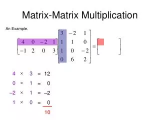
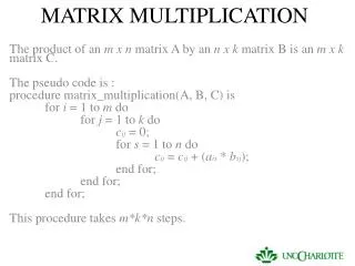
“Naïve” Matrix Multiply {implements C = C + A*B} for i = 1 to n for j = 1 to n for k = 1 to n C(i,j) = C(i,j) + A(i,k) * B(k,j) Algorithm has 2*n3 = O(n3) Flops and operates on 3*n2 words of memory A(i,:) C(i,j) C(i,j) B(:,j) = + * CS267 Lecure 2
“Naïve” Matrix Multiply {implements C = C + A*B} for i = 1 to n {read row i of A into fast memory} for j = 1 to n {read C(i,j) into fast memory} {read column j of B into fast memory} for k = 1 to n C(i,j) = C(i,j) + A(i,k) * B(k,j) {write C(i,j) back to slow memory} A(i,:) C(i,j) C(i,j) B(:,j) = + * CS267 Lecure 2
“Naïve” Matrix Multiply Number of slow memory references on unblocked matrix multiply m = n3 read each column of B n times + n2 read each row of A once + 2n2 read and write each element of C once = n3 + 3n2 So q = f / m = 2n3 / (n3 + 3n2) ~= 2 for large n, no improvement over matrix-vector multiply A(i,:) C(i,j) C(i,j) B(:,j) = + * CS267 Lecure 2
Blocked (Tiled) Matrix Multiply Consider A,B,C to be N by N matrices of b by b subblocks where b=n / N is called the block size for i = 1 to N for j = 1 to N {read block C(i,j) into fast memory} for k = 1 to N {read block A(i,k) into fast memory} {read block B(k,j) into fast memory} C(i,j) = C(i,j) + A(i,k) * B(k,j) {do a matrix multiply on blocks} {write block C(i,j) back to slow memory} A(i,k) C(i,j) C(i,j) = + * B(k,j) CS267 Lecure 2
Blocked (Tiled) Matrix Multiply Recall: m is amount memory traffic between slow and fast memory matrix has nxn elements, and NxN blocks each of size bxb f is number of floating point operations, 2n3 for this problem q = f / m is our measure of algorithm efficiency in the memory system So: m = N*n2 read a block of B, N3 times (N3 * n/N * n/N) + N*n2 read a block of A, N3 times + 2n2 read and write each block of C once = (2N + 2) * n2 So computational intensity q = f / m = 2n3 / ((2N + 2) * n2) ~= n / N = b for large n So we can improve performance by increasing the blocksize b Can be much faster than matrix-vector multiply (q=2) CS267 Lecure 2
Basic Linear Algebra Subroutines • Industry standard interface (evolving) • Vendors, others supply optimized implementations • History • BLAS1 (1970s): • vector operations: dot product, saxpy (y=a*x+y), etc • m=2*n, f=2*n, q ~1 or less • BLAS2 (mid 1980s) • matrix-vector operations: matrix vector multiply, etc • m=n^2, f=2*n^2, q~2, less overhead • somewhat faster than BLAS1 • BLAS3 (late 1980s) • matrix-matrix operations: matrix matrix multiply, etc • m >= 4n^2, f=O(n^3), so q can possibly be as large as n, so BLAS3 is potentially much faster than BLAS2 • Good algorithms used BLAS3 when possible (LAPACK) • Seewww.netlib.org/blas, www.netlib.org/lapack CS267 Lecure 2
BLAS speeds on an IBM RS6000/590 Peak speed = 266 Mflops Peak BLAS 3 BLAS 2 BLAS 1 BLAS 3 (n-by-n matrix matrix multiply) vs BLAS 2 (n-by-n matrix vector multiply) vs BLAS 1 (saxpy of n vectors) CS267 Lecure 2