Ordination in Biological Analyses
Learn how ordination helps answer biological questions, the principles of CANOCO 4.5 analysis, and strategies for starting analyses. Explore patterns in vegetation, biomass, productivity, diversity, and species composition. Uncover the magic of ordination diagrams to interpret data effectively.


Ordination in Biological Analyses
E N D
Presentation Transcript
ORDINATION What is it? What kind of biological questions can we answer? How can we do it in CANOCO 4.5? Some general advice on how to start analyses.
How different or similar is the vegetation at these two places? What are the patterns within each of them? Biomass Productivity Diversity Species composition
Ordination • Analyses of data with many response variables • Search for patterns • We can also quantify and test the effect of one or many predictor variables (tomorrow!!)
A short answer after a long debate: No. Compositional variation in nature tends to be gradual.
How can we analyse species composition? Within some defined environment or area we sample a number of plots and register the species present
SPECIES SPACE Site 1 10 Site 4 Site 5 Tsuga Site 3 Site 2 0 0 10 Pinus
Site space 10 Betula Pine site 2 Tsuga Acer 0 0 10 Site 1
Data dimensions • The sites differ in species abundances • Each species is a variable – a dimension – • in a dataset with n species the differences between plots can be described exactly by their positions in a n-dimensional space • Species are not distributed independently of each other • They respond to the same factors, affect each other… • Can we somehow find a few dimensions that capture the bulk of the compositional information?
Site 1 10 Site 4 Site 5 Tsuga Site 3 Site 2 0 0 10 Pinus
10 Tsuga Site 1 Site 3 Site 4 0 Site 5 0 Site 2 Pinus 10
Site 1 Site 3 Site 4 Site 5 Site 2
This line describes the relative positions of sites along one dimension that captures the largest fraction possible of the variation in species composition We have done a Principal Component Analysis!!!! 10
Linear vs. Unimodal methods • In the examples above we assumed that species abundance and the environment is linearly related • This is sometimes true! (when we are within a ca. 1-2.5 SD ’window’ along an environmental gradient)
Linear vs. Unimodal methods • But what if we want to analyse the whole gradient? • A linear-based method will give a ’wrong’ solution! (which would give us a statistical artifact called the ’horseshoe effect’) • There are unimodal-based methods (CA, DCA, …)
Weigthed average optimum of this species Correspondence analysis (CA)when the response is unimodal Sample where the species is present. (size indicates abundance)
In the same way you can find the optimum of a sample: the weighted average of the species it contains Species present in the sample. (size indicates abundance) Weigthed average optimum of the sample
Weighted averaging • species scores are weighted averages of site scores • the weights are related to how common the species are in the sites • site scores are weighted averages of species scores • the weights are (again) related to how commmon the species are in the sites ITERATIVE METHOD!
The arch problem • After the first CA axis is constructed, the program will start ’looking for’ a second, uncorrelated axis. • If no ’real’ gradient exists in the data, it will tend to ’find’ the folded axis 1 (which by definition uncorrelated, and half the lenght of the first axis)
Identifying the arch problem …and handling it • The problem is easily identified by inspecting • The CA ordination diagram • can you see an arch in the plot positions along axis 2? • The eigenvalues of the first and second axes • Is the eigenvalue of axis 1 ca. 2* that of axis 2) • The problem can be removed by detrending • Detrend by segments in indirect methods
PCA CA The magic behind the ordination diagrams
Biplot interpretation • Species and sample positions along the axes can be presented as ordinaion diagrams • These diagrams tell us something about the species composition the samples • Interpretation differs between ordination diagrams from linear methods (PCA) and unimodal methods (CA)!
PCA Etc.........
Summary • unimodal vs. linear methods • detrending in unimodal methods • biplot vs. centroid interpretation