Download
1 / 44
440 likes | 521 Views
GEOF236 CHEMICAL OCEANOGRAPHY (HØST 2012) Christoph Heinze University of Bergen, Geophysical Institute and Bjerknes Centre for Climate Research Prof. in Global Carbon Cycle Modelling Allegaten 70, N-5007 Bergen, Norway Phone: +47 55 58 98 44 Fax: +47 55 58 98 83

E N D
GEOF236 CHEMICAL OCEANOGRAPHY (HØST 2012) ChristophHeinze University of Bergen, Geophysical Institute and Bjerknes Centre for Climate Research Prof. in Global Carbon Cycle Modelling Allegaten 70, N-5007 Bergen, Norway Phone: +47 55 58 98 44 Fax: +47 55 58 98 83 Mobile phone: +47 975 57 119 Email: christoph.heinze@gfi.uib.no DEAR STUDENT AND COLLEAGUE: ”This presentation is for teaching/learning purposes only. Do not useany material ofthispresentation for any purpose outsidecourse GEOF236, ”Chemical Oceanography”, autumn 2012, Universityof Bergen. Thankyou for yourattention.”
Sarmiento&Gruber 2006 Chapter 2: Tracer conservation and ocean transport, part 2
The tracer conservation equation expresses that changes of ocean water column tracer concentrations depend on the • 3-dimensional ocean velocity field • Biogeochemical sources and sinks • The 3-d velocity field includes a multitude of processes. In general, a quantification of the velocity field is based on a balance of forces and resulting momentum induced on water “parcels”. Advection – convection – mixing – turbulence – wave motion. • The velocity field includes: • Friction forces (windstress, internal friction, bottom and side wall friction) • Pressure gradient forces • Coriolis force (rotating coordinate frame) • Gravity force, buoyancy force • Forcings, drivers: • Wind, evaporation-precipitation, sea ice melt / freezing cooling-warming, tidal force, sea level pressure exerted by atmosphere • Equations/models: • Navier Stokes equations of motion, these are nonlinear and extremely complex • Solutions are provided numerically in ocean general circulation models OGCMs
The wind driven circulation – qualitative findings: Gyres Upwelling/downwelling regions
Surface winds, January: COADS data set Sarmiento & Gruber (2006)
Surface winds, July: COADS data set Sarmiento & Gruber (2006)
Surface winds, schematic pattern of latitudinal variation: Original source: Book of Pond & Pickard, 1983. Sarmiento & Gruber (2006)
Streamlines (isolines of equal velocity) in the upper 50 m of the ocean, “surface currents”: ECCO project, Stammer et al. 2002, dark shades correspond to high velocity Sarmiento & Gruber (2006)
Sea surface height (top) and thermocline currents (0-500m)(bottom): ECCO project, Stammer et al. 2002 Sarmiento & Gruber (2006)
Coastal up and downwelling, southern hemisphere case: Where would you find a typical coastal upwelling in the northern hemisphere? Original: Thurman, 1990 Sarmiento & Gruber (2006)
Open ocean upwelling/downwelling at divergences/convergences: Original: Thurman, 1990 Sarmiento & Gruber (2006)
Large-scale gyre structure of the ocean seen from top, left side shows schematic windstress pattern with latitude variations: Note the westward intensification of ocean currents. Can you give examples for current systems in these west-side currents? Original: Munk & Carrier, 1950 Sarmiento & Gruber (2006)
Sea surface phosphate (annual mean): Original: World Ocean Atlas 2001, Conkright et al 2002
Sea surface nitrate (annual mean): Original: World Ocean Atlas 2001, Conkright et al 2002
SOME THOUGHTS ABOUT THE MAJOR CATEGORIES OF OCEAN CORCULATION: Wind driven circulation Thermohaline circulation – does it exist as such? (think also about continuity equation, conservation of volume) Meridional overturning circulation (MOC)
Sea surface temperatures (annual mean): Original: World Ocean Atlas 2001, Conkright et al 2002 Sarmiento & Gruber (2006)
Sea surface salinities (annual mean): Original: World Ocean Atlas 2001, Conkright et al 2002 Sarmiento & Gruber (2006)
T-S diagram: The isolines indicate equal densities. What dominates density variations at high and low temperatures? Sarmiento & Gruber (2006)
Definitions – thermocline and mixed layer depth: Original: Knauss, 1997, Pickard & Emery 1990 Sarmiento & Gruber (2006)
Potential temperature – global section: Why is the potential temperature shown and not the in situ temperature? Original: WOCE data Sarmiento & Gruber (2006)
Salinity – global section: Original: WOCE data Sarmiento & Gruber (2006)
Source functions of “transient tracers”: Sarmiento & Gruber (2006)
Thermocline ventilation – concept and bomb tritium data: Sarmiento & Gruber (2006)
Thermocline ventilation – formal ages through the “3H/3He tracer clock”: Sarmiento & Gruber (2006)
Strong density variation across the Gulf stream (zonal section): Original: WOCE data Sarmiento & Gruber (2006)
Geostrophic equilibrium – a very much reduced version of the full set of equations of motion:
Radiocarbon age – global meridional cross section: COLOURED VERSION AVAILABLE? Original: GLODAP compilation, Key et al., 2004 Sarmiento & Gruber (2006)
Radiocarbon age – map at 3500 m depth: Original: GLODAP compilation, Key et al., 2004 Sarmiento & Gruber (2006)
Schematic figure of cluster of 8 water molecules Fraction of molecule aggergates as compared to single H2O molecule Sea water T From Dietrich&Kalle, ”Allgemeine Meereskunde”, 1965
Sea water temperature Density maximum From Dietrich&Kalle, ”Allgemeine Meereskunde”, 1965 Freezing point Salinity
From Libes, ”An introduction to marine biogeochemistry”, 1992
What happens to the salt at formation of sea ice ? From Eide, L.I., and S. Martin, The formation of brine drainage features in young sea ice, J. Glaciology, 14(79), 137-154, 1975
From Eide, L.I., and S. Martin, The formation of brine drainage features in young sea ice, J. Glaciology, 14(79), 137-154, 1975
From Eide, L.I., and S. Martin, The formation of brine drainage features in young sea ice, J. Glaciology, 14(79), 137-154, 1975
How to simulate convective overturning or deep water production in models? Non-hydrostatic models (often impractical, require high resolution). Convective adjustment: If shallower layer A gets heavier than layer B. Alternatives: - Homogenisation - Swap vertical position of layers
Model intercomparison for CFC GOSAC report Orr et al., 2002
Model intercomparison for radiocarbon GOSAC report Orr et al., 2002
Meridional global water transport stream function [Sv] from an ocean model (PA2 OGCM, GFDL Princeton): Sarmiento & Gruber (2006)
Meridional Atlantic water transport stream function [Sv] from an ocean model (PA2 OGCM, GFDL Princeton): Sarmiento & Gruber (2006)
Meridional Indo-Pacific water transport stream function [Sv] from an ocean model (PA2 OGCM, GFDL Princeton): Sarmiento & Gruber (2006)
Schematic of the meridional overturning circulation: Original: Toggweiler & Samuals 1993 Sarmiento & Gruber (2006)
Schematic of the global ocean conveyor belt circulation: Original following: Broecker, 1991 and Gnanadesikan&Hallberg, 2002 Sarmiento & Gruber (2006)