Download
1 / 12
120 likes | 245 Views
This guide explores the fundamentals of regression analysis, highlighting the relationship between dependent and independent variables. Starting with the basic algebraic equation of a line, we discuss how the dependent variable (y) relates to the independent variable (x) through concepts like slope and y-intercept. Using a practical example of pizza sales in college towns, we illustrate how data points visualize through scatter plots and regression lines. Learn about the ordinary least squares method for estimating relationships and the significance of error terms in regression models.

E N D
Remember back in your prior school daze some algebra? You might recall the equation for a line as being y = mx + b. Or maybe you had the form y = a + bx. Maybe you even had another form. Did you? Notice how the y term is on the left of the equal sign. It looks like y is all by itself, but actually it is called the dependent variable. The value of y depends on the value of x. x is the independent variable. On the right side the variable x has a coefficient with it called the slope. The slope can be negative or positive, or even zero. The term that is on the right with no x hooked to it is called the y-intercept, or intercept for short. The intercept can be positive, negative or zero.
y This height is called the intercept. x Here I show three different lines with the same intercept. But, different lines could have different intercepts. Intercepts can even be negative.
2 Say we move from a dot one unit away in the x direction. The slope then tells us how far we have to go in the y direction to get back to the line. y 1 The dot on the line is represented by an x value and a y value. ? 1 x 3 Note on the upward sloping (to the right) curve when we went over to the right on x we have to go up on the y variable. On the flat line we wouldn’t move in the y direction at all, and on the downward sloping line we would move down to the line.
Now, in algebra, we might have a specific line with the form • y = 60 + 5x. Then we can say, when • x= y= • 0 60 • 65 • 70 • 75 and so on. In algebra every point fits exactly on the line.
Now, let’s use an example to see how what we have just been thinking about is related to statistics. Say a chain of pizza joints has stores in many college towns. And say it is wondering if the sales in these towns are related to the size of the college in terms of student population. Sales would be the y variable because sales are thought to depend on the population. The student population would be the x variable. On the next screen I have data from 10 of the stores. Note each row is a store and we have on each line the population and the sales. Then we put each store as a dot in the scatter diagram.
Do the dots fit exactly on a line like in algebra? No, but maybe a line can be put into the data so that the line can be used to represent the data.
Math form It is thought that in the population the variable x and y are related in the following general form: y = B0 + B1 x + e, where B0 is the y intercept of the line, B1 is the slope of the line, and e is an error term that captures all those influences on y not picked up by x. The error term reflects the fact that all the points are not directly on the line. So, we think there is a regression line out there that expresses the relationship between x and y. We have to go find it. In fact we take a sample and get an estimate of the regression line.
Later we will see a method to get an estimate, but for now say we have the method. When we have a sample of data from a population we will say in general the regression line is estimated to be ^ y = b0 + b1 x, where the ‘hat’ refers to the estimated value of y. Once we have this estimated line we are right back to algebra. y hat values are exactly on the line. Now, for an each value of x we have data values, called y’s, and we have the one value of the line, called y hat.
At each x a deviation, or residual is the data value minus the y hat value. The method we use to find the line is called the (ordinary) least squares method. From the data of our example I tell you the least squares method gives the equation y hat = 60 + 5x (look like the algebra you saw before?) Now, go back to the slide with the data. Create a y hat, or values of y on the line, column (you don’t have too, but think about it). You get this column by taking the population values for x in each row and plug into the line to get the y hat. The difference between the sales values and the y hat values are the deviations to which I refer.
ordinary least squares The typical method used to pick the line through the data is called the ordinary least squares line. This method is the one that minimizes the sum of squared deviations of the data points to the line. The line has desirable properties(not proven here): 1) It is unbiased - if many samples were taken, the average of the intercepts and slopes from the samples would be the population intercept and slope. 2) It is consistent - ‘large’ samples would give the population intercept and slope as well.
One last point in this section. When you see the scatterplot like the one I had before, you should look at the pattern in the dots. Look at the dots from left to right. 1) if the dots go up hill, suggesting a positive slope, you should get the feel that the sample suggests the relationship between the variables is then beginning to look like a positive relationship – this means the two variables tend to move in the same direction. The means higher values for x go with higher values for y. 2) If the dots go down hill the sample is suggesting there is a negative relationship between the variables. 3) If the dots are flat the sample is suggesting there is no relationship between the variables.